Lecture 1: Basic concepts

What do we plan to cover

Deep learning is changing every day now. So, this is the today list of topics for this course:

• Convolution & Co. Classical CNNs and how do they work
• The pecularities of training deep neural networks (momentum, SGD, loss surfaces, the mystery of generalization).
• CV tasks: object detection, semantic segmentation, transfer learning
• Learning from sequential data: from RNN to Transformer
• Transformer architecture: from NLP back to CV again
• Graph neural networks
• General tricks for efficient training: initialization, data augmentation, compression and pruning, clipping, multi-precision setting, distributed training primitives
• Training of large deep models: checkpointing, offloading, efficient communications, low-precision training.
• Self-supervised learning
• Zero/one-shot learning
• Adversarial attacks and adversarial training.
• Generative models I: Autoregressive models
• Generative models II: Variational autoencoders
• Generative models III: Normalizing flows, NeuralODEs.
• Generative models IV: GAN and score matching.
• Generative models V: Diffusion models.

Homeworks, etc.

We plan to have three homeworks + a project.

Nothing more!

This course is given first time, so any feedback is appreciated (and will be rewarded)

Todays lecture: Basic concepts

• General discussion: how deep learning is different from classical machine learning
• Supervised/unsupervised learning: abstract formulation
• Fully connected neural networks: What it is and why depth matters
• The concept of backpropagation and 'cheap gradients': why it is important to compute the gradient in a fast way (and how)
• Convolutional neural networks: Brief definition of the CNN (to be followed tomorrow)
• Popular deep learning libraries: Tensorflow, Pytorch and Jax.

How deep learning is different from classical machine learning

There is subtle difference between machine learning / deep learning / 'artificial intelligence'.

These terms are now used interchangeably.

Lets try to make some formal definitions.

Machine learning

Machine learning - algorithms that parse data, learn models using these data and make informed decisions or predictions.

It includes linear classifiers, random forests, etc.

Deep learning

The term Deep learning appeared around 1986 (not in the context of neural networks)

and became common around mid-2000.

The first influencial deep learning paper is typically considered to be the paper by Hinton and Salakhutdinov.

It referred mostly to deep neural network models, now used in a broader sense.

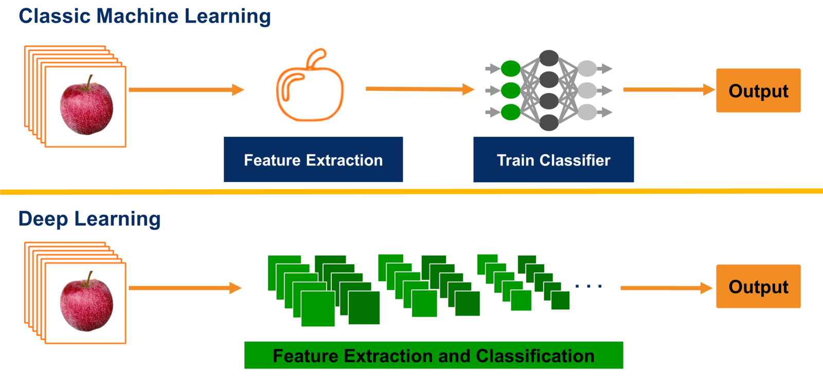
The main idea: hierachical derivation of features for learning.

Awfully incomplete history

• 1943: First artificial neuron by McCulloch and Pitts.
• 1958: Single-layer perceptron: 1958 Rosenblatt perceptron
• 1969: Minsky 'Perceptrons' showed that single-layer has limited capacity (leading to decline in using neural networks).
• 1971: Group method of data handling (Ivakhnenko and Lapa), polynomial models
• 1974: backpropagation (Werbos)
• End of 1980s: LeCun (CNN), RNN
• 1990s: LSTM by Schmidhuber.
• 2012: ImageNet dataset, Krizhevsky et. al show superiority of deep convolutional neural network models
• 2014: Adam, GAN, attention
• 2015: Batchnorm, ResNet
• 2017: Transformer
• 2018: GPT, BERT, ...
• 2020: Vision transformers, diffusion models
• 2021: Self-supervised (CLIP)
• 2022- ChatGPT, GPT-4

Supervised learning

The simplest machine learning model is supervised learning (which you probably already heard about).

You have:

1. A training set $X^{\mathrm{train}} = \{ (x_i, y_i), i=1,\ldots, N$ }, and a test set $X^{\mathrm{test}} = \{ (\tilde{x}_j, \tilde{y}_j), j=1,\ldots, M$ },
2. A loss function $l(y, \hat{y})$ that measures how accurate is the prediction $\hat{y}$ for a particular sample.
3. A machine learning model $\hat{y} = f(x, \theta)$, defined by certain parameters $\theta$

This can be regression, binary classification or multiclass classification in the simplest cases.

The vectors $x_i$ are called features of the object. Feature engineering and selection of the model class is one of the crucial tasks of an ML/DS expert.

We want the model to generalize: good train accuracy, and good test accuracy. This is achieved by:

• Train/test splitting (no difference between train test, sampled i.i.d)
• Model architecture (should be appropriate for the task)
• Optimization method (should avoid 'badly generalizable' minima)

Abstract problem formulation

Thus, in supervised learning our goal is to minimize the loss function

$$g(\theta) \rightarrow \min, \quad g(\theta) = \frac{1}{N} \sum_{i=1}^N l(y_i, \hat{y}_i), \quad \hat{y}_i = f(x_i, \theta).$$

Looks like a general optimization problem.

Question: Does this optimization problem have any special structure, which we can use?

Loss functions

Thus, in supervised learning our goal is to minimize the loss function

$$g(\theta) \rightarrow \min, \quad g(\theta) = \frac{1}{N} \sum_{i=1}^N l(y_i, \hat{y}_i), \quad \hat{y}_i = f(x_i, \theta).$$

Possible choices of the loss function:

1. Mean squared error (MSE):

$$l(y, \hat{y}) = \frac{1}{2}(y - \hat{y})^2$$

2. For binary classification, we can use binary cross entropy (we assume that the output $\hat{y} \in [0, 1]$).

$$l(y, \hat{y}) = -y\log(\hat{y}) - (1-y)\log(1-\hat{y})$$

3. For multiclass classification we can use cross entropy:

$$l(y, \hat{y}) = -\sum_{c=1}^Cy_c\log(\hat{y}_c)$$

where $y$ is a one-hot encoded vector of true labels, $\hat{y}$ is the predicted class probabilities, and $C$ is the number of classes.

Unsupervised learning

The goal of unsupervised learning is to extract patterns from the data without exact labels to predict.

We have to invent loss functions for different tasks.

One of the most common settings is to model the probability distribution $p(x)$ of the observed data,

and maximize the likelihood

$$g(\theta) = \frac{1}{N} \sum_{i=1}^N \log p(x_i, \theta).$$

Other type of unsupervised learning include constrastive learning, clustering.

Deep learning architectures

The parametrization of the model $f(x, \theta)$ is the key ingredient.

The standard approach of 'classical' machine learning is to design a certain map $E(x)$ with comes from the expert knowledge.

Then, learn a simple (i.e., linear) model

$$y = f(E(x), \theta)$$

.

The concept of end-to-end learning is to avoid predesigned feature engineering, rather than consider parametric building blocks, and learn them simultaneously.

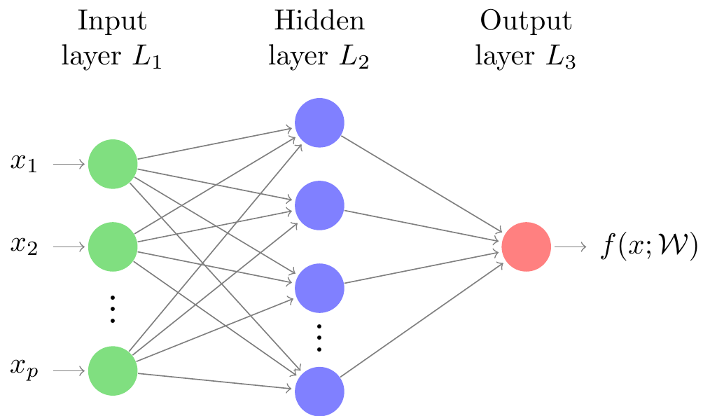
The simplest representation of this form is feedforward neural networks.

Fully connected neural networks

The basic deep learning model is the feedforward model neural network (also known as multilayer perceptron, MLP).

Mathematically, it is a superposition of linear and simple non-linear transformations:

$$f(x) = f_k(f_{k-1}(\ldots (f_0(x))),$$

where

$$f_k(x_k) = \sigma( W_k x_k + b_k)$$

is one layer of the transformation.

$W_k$ is an $r_{k} \times r_{k-1}$ matrix (called weight), $b_k$ is a vector of length $r_k$ called bias,

$\sigma$ is a pointwise nonlinearity function (sigmoid, or ReLU).

Popular non-linearities

1. Sigmoid: The sigmoid function maps any real-valued number to a value between 0 and 1, making it useful for binary classification problems. It is defined as:

   $$\sigma(x) = \frac{1}{1 + e^{-x}}$$

2. ReLU (Rectified Linear Unit): The ReLU activation function is defined as the positive part of its argument, i.e., $f(x) = \max(0, x)$. It has become popular because of its simplicity and effectiveness in deep neural networks.

3. Leaky ReLU: The Leaky ReLU is similar to ReLU, but allows for a small, non-zero gradient when the input is negative. It is defined as:

   $$f(x) = \begin{cases} x, & \text{if } x > 0 \\ ax, & \text{otherwise} \end{cases}$$

   where $a$ is a small positive constant.

4. Tanh (Hyperbolic Tangent): The tanh function maps any real-valued number to a value between -1 and 1. It is defined as:

   $$\tanh(x) = \frac{e^{x} - e^{-x}}{e^{x} + e^{-x}}$$

5. Sine: The sine function can be used as an activation function, especially in audio-related tasks. It is defined as:

   $$\sin(x)$$

6. SELU (Scaled Exponential Linear Unit): The SELU activation function is a self-normalizing activation function that outputs zero mean and unit variance activations, helping to reduce the internal covariate shift problem. It is defined as:

   $$f(x) = \lambda \begin{cases} x, & \text{if } x > 0 \\ \alpha(e^x - 1), & \text{otherwise} \end{cases}$$

   where $\alpha$ and $\lambda$ are constants determined from the mean and variance of the input data.

7. Swish: The Swish activation function is a recently introduced activation function that has shown promising results in deep learning. It is defined as:

   $$f(x) = x\sigma(\beta x)$$

   where $\sigma$ is the sigmoid function and $\beta$ is a hyperparameter.

What MLP can approximate: Depth

Why do we need deep networks?

This is the concept of expressive power: deep networks reprsent much broader class of functions.

Meta-theorem: If we have a random feed-forward deep network, in order to represent it exactly with a shallow network we need exponentially large width.

## Building neural network
import torch
import torch.nn as nn
# Define the model architecture
input_size = 1
hidden_size = 10
output_size = 1
model = nn.Sequential(
    nn.Linear(input_size, hidden_size),
    nn.ReLU(),
    nn.Linear(hidden_size, output_size),
)

x0 = torch.linspace(-1, 1, 256)
print(x0.shape)
#y = model(x0) #Will be an error, why?

torch.Size([256])

#!pip install graphviz
#conda install --channel conda-forge pygraphviz
#!pip install torchview
#https://github.com/mert-kurttutan/torchview
from torchview import draw_graph

batch_size = 5
# device='meta' -> no memory is consumed for visualization
model_graph = draw_graph(model, input_size=(batch_size, 1), device='meta')
model_graph.visual_graph

What MLP can approximate

There is a famous Universal Approximation Theorem by Cybenko (1989) and Hornik et al. (1989).

Let $f: \mathbb{R}^n \rightarrow \mathbb{R}$ be a continuous function. Then $f$ can be approximated arbitrarily well by a neural network with a single hidden layer, if and only if the activation function of the network is a continuous, non-constant, and bounded function that is not a polynomial.

Deep networks

The problem of universal approximation theorem is that the width can be exponentially large for good approximation.

Can depth help for the approximation of simple functions?

• Theoretically: Yes (see the pionering work by Dmitry Yarotsky)
• Practically: For regression depth does not help at all.

For image processing/Natural Language Processing (NLP) the depth of deep neural network helps a lot.

The concept of backpropagation and 'cheap gradients'

The most straightforward optimization method will be gradient descent.

$$g(\theta) \rightarrow \min, \quad g(\theta) = \frac{1}{N} \sum_{i=1}^N l(y_i, \hat{y}_i), \quad \hat{y}_i = f(x_i, \theta).$$$$\theta_{k+1} = \theta_k - \alpha \nabla_{\theta} g. $$

Parameter $\alpha$ is called learning rate for training, it also may depend on the step $\alpha = \alpha_k$ (this will be known as learning rate schedule).

Note, that it was not the first idea to use gradient descent for feed-forward networks!

Such things as sequential learning, or second-order methods have been tried many times.

How to compute the gradient in a cheap way?

Given $$ g(\theta) = \frac{1}{N} \sum_{i=1}^N l(y_i, \hat{y}_i), \quad \hat{y}_i = f(x_i, \theta).$$ how to compute the gradient in a cheaper way?

I need at least two answers!

Recipe to speed up 1: Stochastic gradient descent

Instead of summing over all dataset, randomly pick a subset (called batch) and evaluate the gradient on it:

$$\nabla g(\theta) \approx \frac{1}{B} \sum_{k=1}^B \nabla_{\theta} l(y_{i_k}, \hat{y}_{i_k}), \quad \hat{y}_{i_k} = f(x_{i_k}, \theta).$$

Obvious: The complexity of a gradient is reduced by a factor of $\frac{N}{B}$.

Not obvious: Stochastic gradient descent (SGD) leads to completely different convergence than ordinary gradient descent.

But still, how to compute the gradient for a single sample of the dataset?

A good deep learning model may have hunderds of millions of parameters even if it is small...

Recipe to speed up 2: Computing the gradient of a function

Our function is given as a superposition of simple functions.

It depends on many parameters.

Does the complexity of the evaluation of the gradient depends on the number of variables?

(I.e. if the model has $P$ parameters, we need to compute $P$ values).

Baur-Strassen theorem (1983) says (informally) that for almost any computer code:

If $g(\theta)$ takes $K$ flops to evaluate, we can generate an algorithm that compute $\nabla_{\theta} g$ in $cK$ flops, where $c$ is a constant.

Downside: We may need a lot of additional memory!

Backpropagation: fast evaluation of the gradient

We can use chain rule for feedforward models:

$$l(y, f(x, \theta)) = l(y, f_2(f_1(x, \theta_1), \theta_2)),$$

How we compute the gradient with respect to $\theta_2$?

$$\frac{\partial g}{\partial \theta_2} = \left(\frac{\partial f_2}{\partial \theta_2}\right)^{\top}\frac{\partial l}{\partial \hat{y}}$$

With respect to $\theta_1$ we need to compute the gradient of $f_2$ with respect to the input.

I.e., we first compute the vector $v_2 = \frac{\partial l}{\partial \hat{y}}$.

Then we compute

$$v_1 = \left(\frac{\partial f_2}{\partial x_2}\right)^{\top} v_2 $$

Then we compute

$$\frac{\partial g}{\partial \theta_1} = \left(\frac{\partial f_1}{\partial \theta_1}\right)^{\top} v_1$$

Reverse mode differentiation

• PyTorch and Jax by default use reverse mode differentiation, which we just described (i.e. for each computational block we need to implement transposed Jacobian-by-vector product).

• There is also a forward mode differentiation.

• In forward mode, we compute the derivatives simultaneously with the value.

• Reverse mode and forward mode are two extreme ways of traversing the chain rule for the derivatives.

Idea of forward mode differentiation using dual numbers

We introduce dual numbers. A dual number has the form $x + \varepsilon x'$ and $\varepsilon^2 = 0.$

The connection to differentiation can be seen from formal Taylor series:

$$f(x + \varepsilon x') = f(x) + \varepsilon f'(x). $$

For the vector case, we have $P$ numbers $\varepsilon_i$ and they satisfy $\varepsilon_i \varepsilon_j = 0$.

If the number of input variables is small, forward mode will be much faster!

Automatic differentiation (advanced)

One can show:

• Optimal AD is NP-complete task
• One can reduce the problem of computing the gradient to the computation of the column of the inverse of the lower-triangular linear system.

Transposed Jacobian-by-vector for simple layers: linear layer

Let $y = f(x, W) = Wx$ be the linear transform. Then the transposed Jacobian times vector for a single sample has the following form:

• $\left(\frac{\partial y}{\partial W}\right)^{\top} o = xo^{\top},$

• $\left(\frac{\partial y}{\partial x}\right)^{\top} o = W^{\top}o,$

where $o = \frac{\partial g}{\partial y}$ comes from backpropagation.

Transposed Jacobian-by-vector for simple layers: nonlinearity

Let $y = \sigma(x)$, then we need to compute

$$ \frac{\partial y}{\partial x} o = \sigma'(x) \circ o, $$

i.e. we need to compute the derivative of $\sigma$ and do elementwise multiplication with the vector $o$ that comes from backpropagation.

Storage

Consider MLP. Then, computation of the gradient requires:

1. Storing all intermediate computation before linear layer and before non-linearity (forward pass).
2. Compute transposed Jacobian matrix-by-vector product (backward pass).

In inference, we don't need to store intermediate values ($x_k$, also called activations).

Inference can be initiated as

with torch.no_grad():
    model(x)

But no gradients can be computed in this case!

## Building neural network
#%pip install -U git+https://github.com/szagoruyko/pytorchviz.git@master
from torchviz import make_dot, make_dot_from_trace
import torch
import torch.nn as nn
# Define the model architecture
    
input_size = 1
hidden_size = 10
output_size = 1
model = nn.Sequential(
    nn.Linear(input_size, hidden_size),
    nn.ReLU(),
    nn.Linear(hidden_size, output_size),)
model.to(device)

    
x = torch.linspace(-2, 2, 256)
x = x[:, None]
y = x**2

def compute_loss(model, x, y):
    #with torch.no_grad():
    #    er = y - model(x)
    #    loss = torch.mean(er**2)
    er = y - model(x)
    loss = torch.mean(er**2)
    
    return loss
make_dot(compute_loss(model, x, y), params=dict(model.named_parameters()))

Convolutional neural networks (1)

For image processing, one of the most efficient architecture is the convolutional neural network (CNN)

First CNN have been feedforward.

The main difference is how the linear layer is implemented.

In MLP, we have

$$x_{k+1} = \sigma(W_k x_k + b_k)$$

and $W_k$ is a dense matrix.

If $x$ is an image, it can be treated a three-dimensional array $X \times Y \times S$ (width-height-channels).

Convolutional neural networks (2)

If we have say $224 \times 224 \times 3$ image, we will need to store a $150528 \times 150528$ matrix, which is impossible.

In classical image processing, many transformations are given in the form of convolutions.

Reminder:

The most ``important" and time-consuming operation within modern CNNs is the generalized convolution that maps an input tensor $U(\cdot, \cdot, \cdot)$ of size $X \times Y \times S$ into an output tensor $V(\cdot, \cdot, \cdot)$ of size $(X - d + 1) \times (Y - d + 1) \times T$ using the following linear mapping:

$$V(x, y, t) = \sum_{i=x-\delta}^{x+\delta} \sum_{j=y-\delta}^{y+\delta} \sum_{s=1}^S K(i - x + \delta, j - y + \delta, s, t) U(i, j, s)$$

CNN, complexity

$$V(x, y, t) = \sum_{i=x-\delta}^{x+\delta} \sum_{j=y-\delta}^{y+\delta} \sum_{s=1}^S K(i - x + \delta, j - y + \delta, s, t) U(i, j, s)$$

The size of the filter determines the number of pixels in the window (here - $\delta$).

If $\delta$ is small, one can use this formula directly, resulting in $\delta^2 XY ST$ complexity. No need to store the full layer!

If $\delta$ is large, one can use Fast Fourier Transform (FFT).

Nowdays, it is even popular to use 1x1 convolution and depth-wise convolutions (which are not really convolutions).

We will discuss these architectures in more detail tomorrow.

CNN: the architecture

We will discuss CNN tomorrow, including a very important pooling layer (which made it possible to learn on the so-called ImageNet dataset).

Popular deep learning libraries

The main deep learning libraries available now are Tensorflow, Pytorch and Jax.

Lets discuss them.

Tensorflow

• TensorFlow is an open-source platform for building and deploying machine learning models.
• Developed by Google and released in 2015.
• Provides both high-level APIs for building and training models quickly and low-level APIs for more control and flexibility.
• Provides a flexible architecture to support a variety of deployment scenarios, including on-premises, cloud-based, and mobile devices.
• TensorFlow has a large and active community, with a vast range of resources and tutorials available online.
• The latest version of TensorFlow is TensorFlow 2.0, which has improved ease-of-use and performance compared to previous versions.
• TensorFlow also provides tools for visualizing and debugging models, such as TensorBoard.
• TensorFlow has support for both CPU and GPU acceleration, allowing for efficient training and inference on a wide range of hardware.

Pytorch

• Pytorch is an open-source platform for building and deploying machine learning models.
• Developed by Facebook and released in 2018.
• Dynamic computational graph, easy for debugging and its own memory management
• Huge community, the most popular in academia (a lot of pretrained models/code)
• Current version is Pytorch 2.0 which is focused on speed (i.e., it has torch.compile)
• CPU/GPU support
• Distributed training

Jax

• Jax has become quite popular recently, developed by Google in 2018
• JAX uses a functional programming model that enables users to express complex numerical computations as pure functions that can be composed, transformed, and optimized for efficient execution. jax.jit, jax.grad, jax.vmap (vectorization), recently similar functionality appeared in Pytorch
• JAX is designed to work seamlessly with NumPy, allowing users to take advantage of the vast ecosystem of scientific computing tools available in Python.
• JAX is built for performance and scales well on modern hardware, including CPUs, GPUs, and TPUs.
• It supports distributed computing and can be used to train large-scale models efficiently.
• Quite a few problems if you move from Pytorch

Comparison

Tensorflow	Jax	Pytorch
+ Widely used in industry and academia	+ Designed for high-performance numerical computing	+ Dynamic computational graph allows for flexibility
+ Large and active community with extensive documentation	+ Automatic differentiation for fast and efficient gradient computation	+ Supports various neural network architectures
+ Supports distributed computing for large-scale training	+ Supports GPU and TPU acceleration	+ Easy to use and learn
- Can have a steep learning curve for beginners	- Smaller community compared to other frameworks	- Some operations can be slower than other frameworks
- Code can be verbose and difficult to read	- Functional programming knowledge needed	- Debugging can be difficult

Some hints

If the goal is to train a known model on a given dataset, no big difference (Pytorch and Tensorflow have better dataset handling).

If we need speed, Jax is a good option.

Overall, it is a matter of taste, and the difference between frameworks has become not so evident.

So, what is deep learning?

End-to-end joint learning of all layers:

• multiple assemblable blocks (“modules”)

• each block is piecewise-differentiable

• gradient-based learning from examples

• gradients computed by backpropagation

Take home message

• Supervised learning
• Basic idea of automatic differentiation (forward/reverse mode)
• Fully connected networks
• Three main libraries

Next lecture

Convolutional neural networks in more details:

• Motivation of using convolutions (and connection to classical image processing)
• Basic building blocks of a CNN (convolutions in 1D, 2D, 3D, pooling)
• Convolutions and (equivariance)
• Overview of the main architectures (LeNet, AlexNet, VGG, ResNet, Inception)
• Visualization of learned filters