Lecture 10: Contrastive learning / self-supervised learning
Previous lecture: General tricks for efficient training:
- checkpointing
- offloading
- efficient communications
- low-precision training.
Current lecture: Contrastive learning / self-supervised learning
- What is contrastive learning
- Popular losses
- SimCLR
- MoCo
- ByOL
- Barlow Twins
- VicReg
What is constrastive learning
Constrastive learning is a technique, where you have a lot of unlabeled data (typically, it is related to images).
We want to learn an encoder $x \rightarrow E(x)$ such that we can distinguish positive and negative samples.
Contrastive learning is a special class of self-supervised learning.
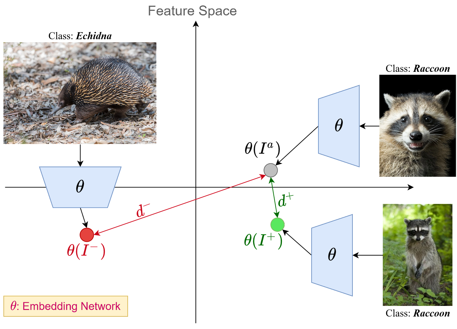
Constrastive learning
We select a data sample (sometimes called anchor), the data point belonging to the same distribution as anchor,
and a negative sample.
An SSL model tries to minimize the distance between anchor and positive sample, while simultaneously maximizing the distance between positive samples and negative samples.
The distance can be measured in many different ways.
How to find positive and negative samples?
There are several methods to find positive-negative samples.
There are many ways to measure distances.
The standard approach is to apply image transformations to the anchor image and use those as positive samples.
We can use standard augmentations covered in our class on it, typically:
color jitter, rotation, flipping, noise, random affine.
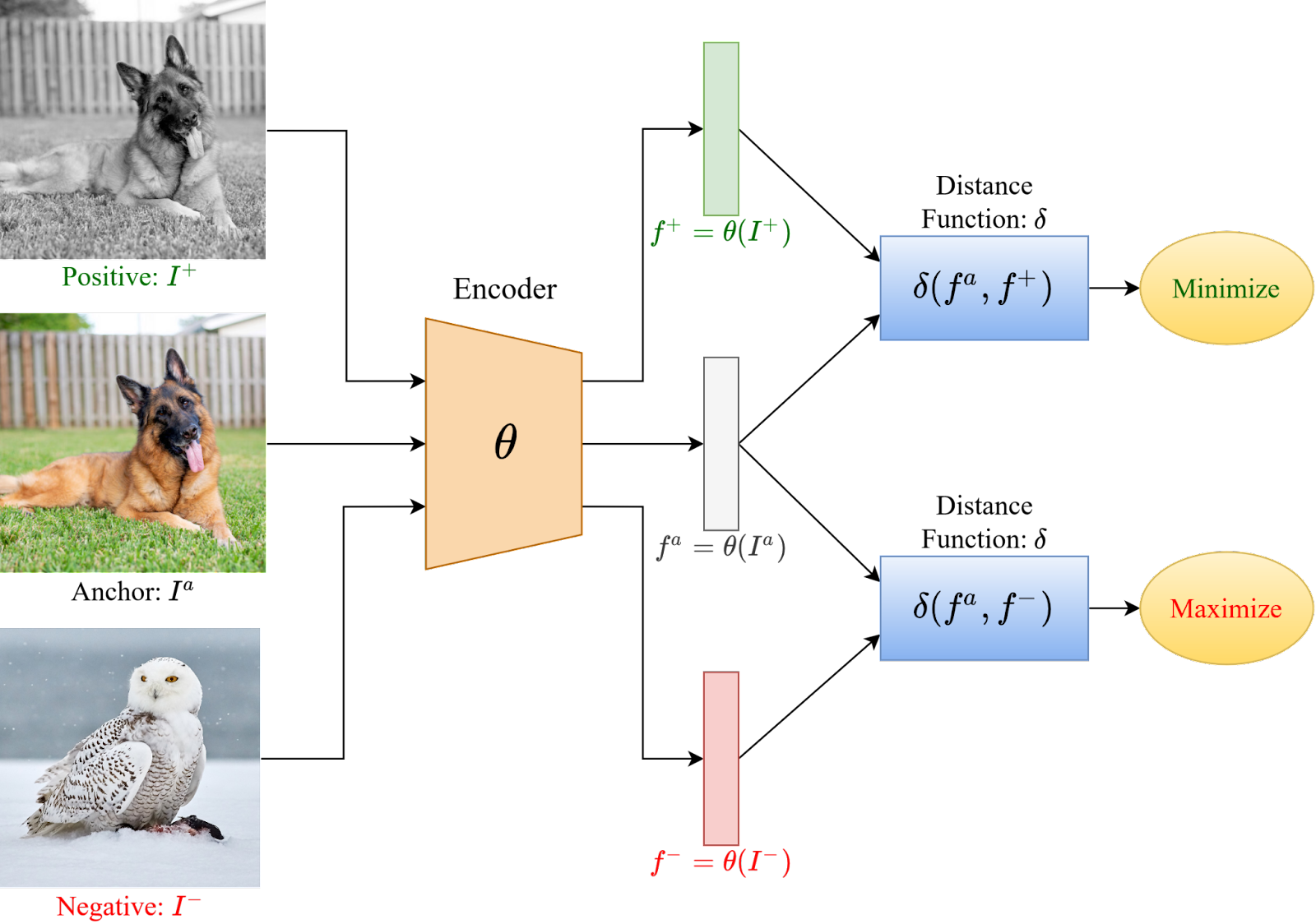
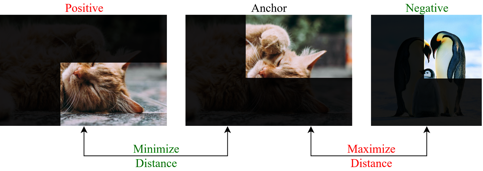
Image patches
The second approach is to break image into patches.
Use patches from the same image as positive, from others as negative.
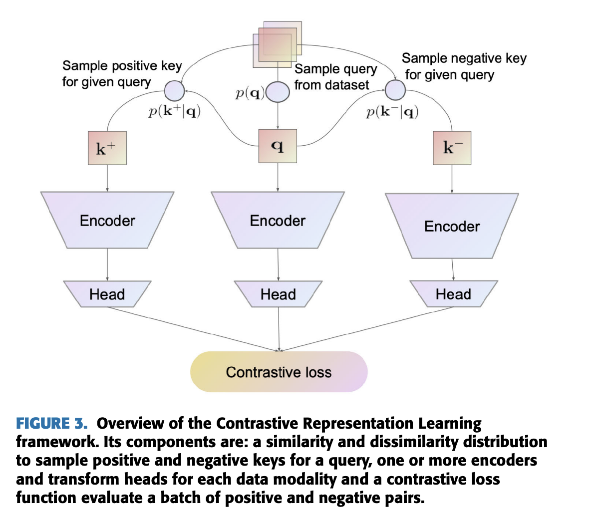
Objectives
We have a query $q$, positive key $k^+$ and negative key $k^-$. We need to introduce the notions described above.
This can be done by using several losses:
- Max margin contrastive loss
- Triplet loss
- Info NCE
- NT-Xent Loss
Max-margin contrastive loss
The first loss was proposed by Chopra, Hadsell, and LeCun in 2006, and was motivated by so-called energy models.
Specifically, it has the form
$$ L_{\mathrm{pair}} = \begin{cases} D(q, k)^2, & k \sim p^+(\cdot \vert q) \\ \max(0, m - D(q, k)^2) &k \sim p^-(\cdot \vert q) \end{cases}$$The distance between positive pairs is minimized, between negative it is maximized.
Triplet loss
Triplet loss had a strong impact in FaceId systems, where contrastive approaches are very efficient
It is given as
$$L(q, k^+, k^-) = \max(0, D(q, k^+)^2 - D(q, k^-)^2 + m)$$Probabilistic losses
$$p(k^+|q) = \frac{\exp(q^{\top} k^+)}{\sum_{k \in \mathcal{K}} \exp(q^T k)} = \frac{\exp(q^{\top} k^+)}{Z(q)}.$$The normalization constant is hard to evaluate: we need to sum over all negative samples in the dataset for the given query.
The original NCE (noise contrastive estimation) assume a uniform distribution of the negative samples for a given query.
Then, if we sample $m$ times more often the negative sample, we get the following value ($D=1$ corresponds to the positive distribution) $$p(D = 1|q, k) = \frac{p(k^+ \vert q)}{p(k^+\vert q) + m \cdot p(k^- \vert q)}$$
First idea
The first idea has been done in the paper Dimensionality Reduction by Learning an Invariant Mapping Raia Hadsell, Sumit Chopra, Yann LeCun in 2006,
With the idea of learning representations that are invariant to certain transformations.
Later techniques
Several techniques have been proposed later.
One is Contrastive predictive coding where autoregressive models are used for prediction.
One can also think about BERT-type masking as contrastive learning, but it requires additional visual token encoders, which map images to visual tokens.
We basically predict the missing part given the rest.
Different approaches
There are different approaches where do we get positive/negative samples.
We can have a memory bank that stores the negative samples, and train using it. It requires additional memory.
There are alternative approaches.
We will discuss the most popular ones.
Memory bank idea
Instead of the softmax classifier, we consider a non-parametric version of it, where $v_i$ are prototypes.
We will talk about prototypes when we will take about one-shot / few-shot learning.
$$P(i \vert v) = \frac{\exp(v^{\top}_i v/\tau)}{\sum_{j=1}^n \exp(v^{\top}_j v/\tau)}$$All features for each object is stored in the memory bank. When the model is updated, the features are updated as well.
If we have millions of classes using full softmax is prohibited, thus NCE can be used.
More discussion is in this paper
SimCLR
SimCLR is a framework, which is built on a general principles from certain modules.
- Stochastic data augmentation module: transforms any given data sample randomly, giving two different views $\hat{x}_i$ and $\hat{x}_j$. These are two correlated views of the same image. We consider this as a positive pair.
- Base encoder (given as a neural network). Can be ResNet or transformer module.
- A small projection head that maps the input to the space where the contrastive loss is applied. A simple 1-layer network is used.
SimCLR: continued
Suppose we have $N$ sample. We generate $2N$ by augmentation. We think we have one positive pair and $2N-2$ negative pairs. Thus we may introduce a loss function as
$$l_{ij} = -\log\frac{\exp(\text{sim}(z_i,z_{j})/\tau)}{\sum_{k=1}^{2N}[k\neq i]\exp(\text{sim}(z_i,z_k)/\tau)}$$where $$\mathrm{sim}(u, v) = \frac{(u, v)}{\Vert u \Vert \Vert v \Vert}$$
is the cosine similarity between vectors $u$ and $v$.
This loss has been used before (called NT-Xent).
We need to sum over all pairs $i, j$.
Facts from the paper:
- The model is trained with large batch sizes.
- Much stronger augmentation is needed compared to supervised learning, in the end they settled down with simple cropping and color.
MoCo
We can look at the contrastive learning as dictionary lookup task.
We have an input query q and $\{k_0, k_1, k_2, \ldots, \}$ are the encoded samples.
A contrastive loss is a function that is low when $q$ is close to its positive pair $k_{+}$ are far from all other keys.
MoCo uses $$L_q = -\log \frac{\exp((q \cdot k_+)/\tau)}{\sum_{i=0}^K \exp((q \cdot k_i)/\tau)},$$
the sum is over $K$ negative samples
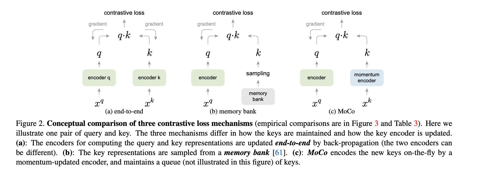
MoCo, continued
The dictionary is kept large, the encoder is updated but not trained, but it is smoothed as
$$\theta_k = m \theta_k + (1-m) \theta_q,$$where $m = 0.999$
# f_q, f_k: encoder networks for query and key
# queue: dictionary as a queue of K keys (CxK)
# m: momentum
# t: temperature

f_k.params = f_q.params # initialize

for x in loader: # load a minibatch x with N samples
    x_q = aug(x) # a randomly augmented version
    x_k = aug(x) # another randomly augmented version
    q = f_q.forward(x_q) # queries: NxC
    k = f_k.forward(x_k) # keys: NxC
    k = k.detach() # no gradient to keys

    # positive logits: Nx1
    l_pos = bmm(q.view(N,1,C), k.view(N,C,1))
    # negative logits: NxK
    l_neg = mm(q.view(N,C), queue.view(C,K))
    # logits: Nx(1+K)
    logits = cat([l_pos, l_neg], dim=1)
    # contrastive loss, Eqn.(1)
    labels = zeros(N) # positives are the 0-th
    loss = CrossEntropyLoss(logits/t, labels)
    # SGD update: query network
    loss.backward()
    update(f_q.params)
    # momentum update: key network
    f_k.params = m*f_k.params+(1-m)*f_q.params
    # update dictionary
    enqueue(queue, k) # enqueue the current minibatch
    dequeue(queue) # dequeue the earliest minibatch.
MoCo version 2
Some architectural ideas borrowed from SimCLR that improve the accuracy!
- Replace FC head with 2-layer MLP head
- Add blur augmentation
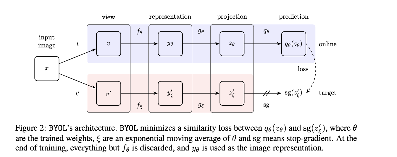
Bootstrap your Latent (BYOL)
Bootstrap Your Own Latent - A New Approach to Self-Supervised Learning
In BYOL, two networks are used. They are referred to as online and target networks, that interact and learn from each other.
The network weights $\xi$ are update after each training step as
$$\xi := \tau \xi + (1-\tau) \theta).$$The motivation behind is quite vague, but the SOTA numbers were obtained!
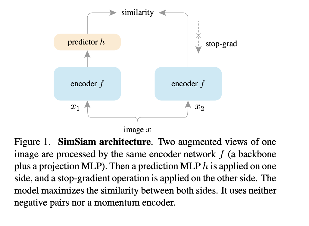
Simple Siamese networks
Exploring Simple Siamese Representation Learning
One can share two networks and just update them:
Barlow twins
One can also try the objective to make the representations uncorrelated, as done in Barlow Twins: Self-Supervised Learning via Redundancy Reduction
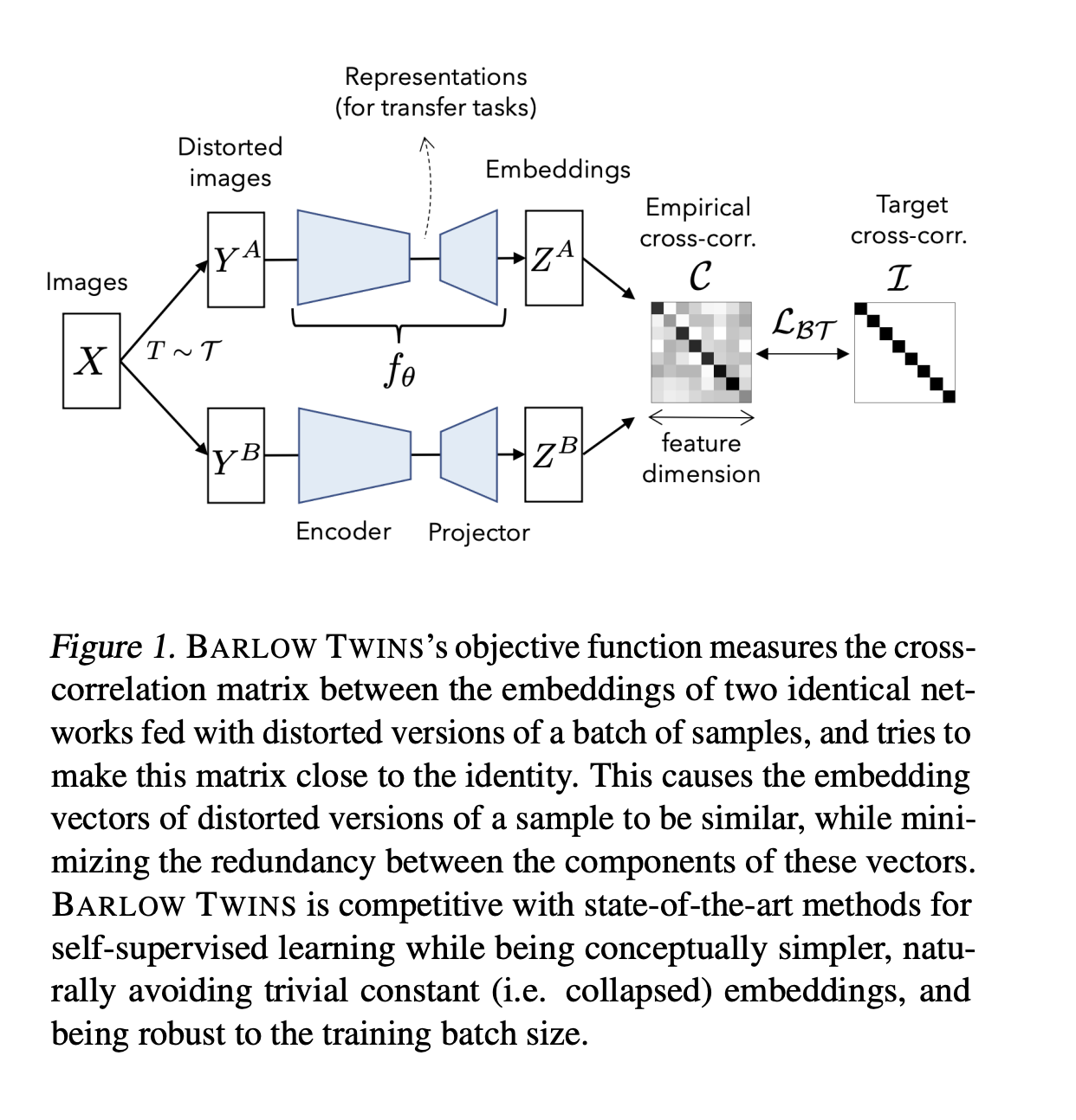
Barlow-twins
Barlow twins naturally avoids the collapse problem by requiring the two views be completely uncorrelated.
I.e., we augment the data two times (two views of the dataset) and then we require that the correlation between those is close to $1$.
# f: encoder network
# lambda: weight on the off-diagonal terms
# N: batch size
# D: dimensionality of the embeddings
#
# mm: matrix-matrix multiplication
# off_diagonal: off-diagonal elements of a matrix
# eye: identity matrix
for x in loader: # load a batch with N samples
    # two randomly augmented versions of x
    y_a, y_b = augment(x)
    # compute embeddings
    z_a = f(y_a) # NxD
    z_b = f(y_b) # NxD
    # normalize repr. along the batch dimension
    z_a_norm = (z_a - z_a.mean(0)) / z_a.std(0) # NxD
    z_b_norm = (z_b - z_b.mean(0)) / z_b.std(0) # NxD
    # cross-correlation matrix
    c = mm(z_a_norm.T, z_b_norm) / N # DxD
    # loss
    c_diff = (c - eye(D)).pow(2) # DxD
    # multiply off-diagonal elems of c_diff by lambda
    off_diagonal(c_diff).mul_(lambda)
    loss = c_diff.sum()
    # optimization step
    loss.backward()
    optimizer.step()
Vic-Reg
Another approach proposed in VICReg: Variance-Invariance-Covariance Regularization for Self-Supervised Learning
The goal is to avoid some special tricks with mode collapse.
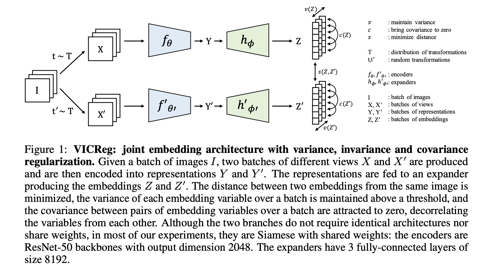
VicReg: the loss
There are 3 losses:
Invariance: the mean square distance between the embedding vectors.
Variance: a hinge loss to maintain the standard deviation (over a batch) of each variable of the embedding above a given threshold. This term forces the embedding vectors of samples within a batch to be different.*
Covariance: a term that attracts the covariances (over a batch) between every pair of (centered) embedding variables towards zero. This term decorrelates the variables of each embedding and prevents an informational collapse in which the variables would vary together or be highly correlated.
The losses are quite complicated and can be found in the paper itself
A cool property is that modalities of the branches can be different.
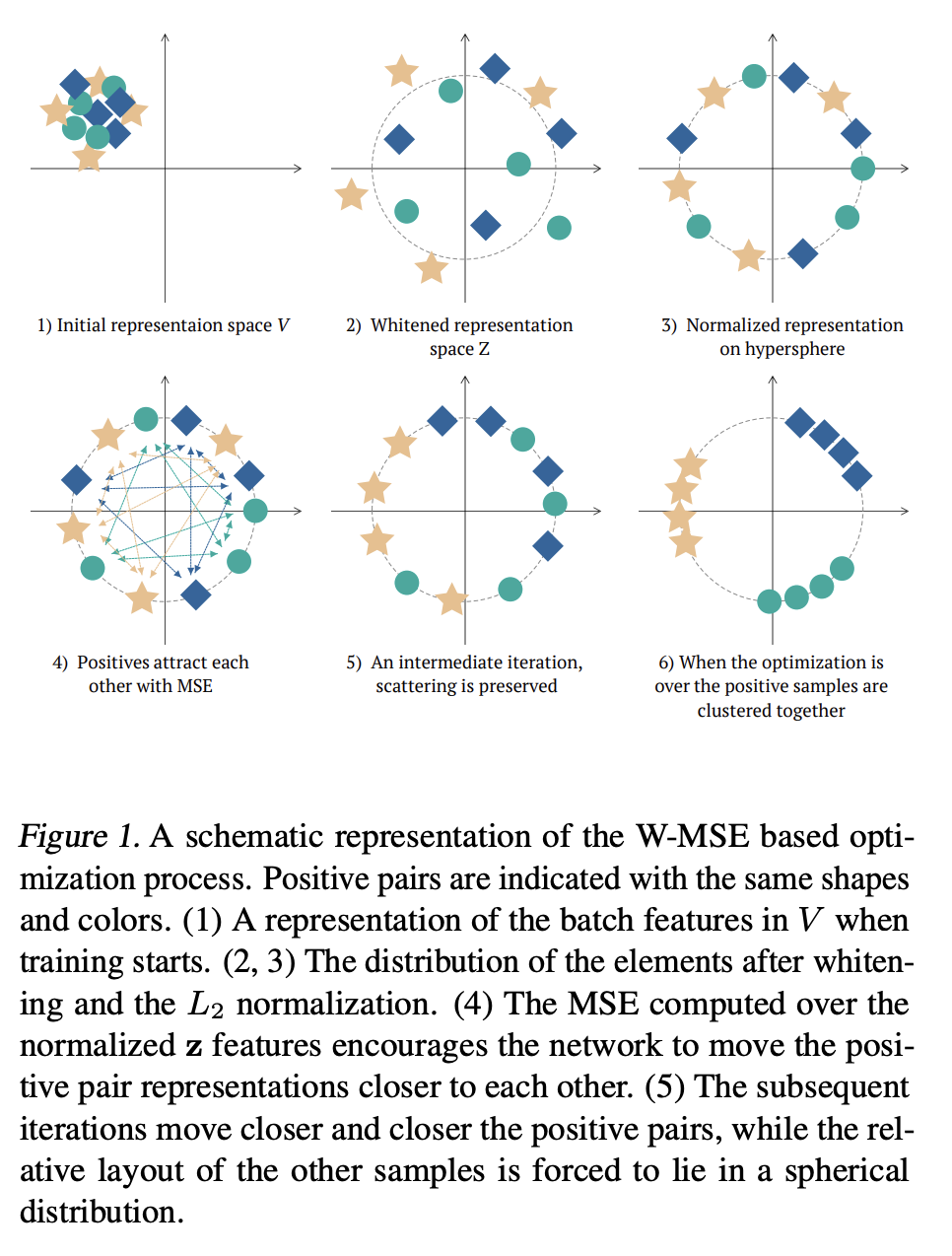
Contrastive Whitening
A very nice (but theoretically not explained!) idea has been proposed in Whitening for Self-Supervised Representation Learning, Aleksandr Ermolov, Aliaksandr Siarohin, Enver Sangineto, Nicu Sebe
Again, we generate augmentations.
We have positive pair $(x_i, x_j)$ and we want to learn a mapping $z = f(x, \theta)$ such that
$$E \mathrm{dist}(z_i, z_j) \rightarrow \min, \quad \mathrm{cov}(z_i, z_j) = I.$$Constrastive Whitening
The orthogonalization is implemented to avoid mode collapse. Note, that you need to differentiate through QR here (in the paper is implemented through regularized Cholesky decomposition)
Interpretation as spectral clustering
Can we find any theoretical justification of what is going on here?
The simplest case would be augmentation with Gaussian noise.
Let $u$ be the mapping, and we are looking for a $1D$ embedding first.
Then, we will have to minimize
$$ E_{x, \varepsilon} \Vert u(x + \varepsilon) - u(x) \Vert^2. $$Let $\varepsilon \sim N(0, \sigma^2)$, then this has a limit for $\sigma \rightarrow 0$!
Interpretation as spectral clustering
We will have the following optimization:
$$\int \rho \Vert \nabla u \Vert^2 dx \rightarrow \min, \, \mbox{s.t.} \int \rho u^2 = 1, \int \rho u = 0$$This is leading eigenvalue of the weighted Laplacian operator on the manifold!
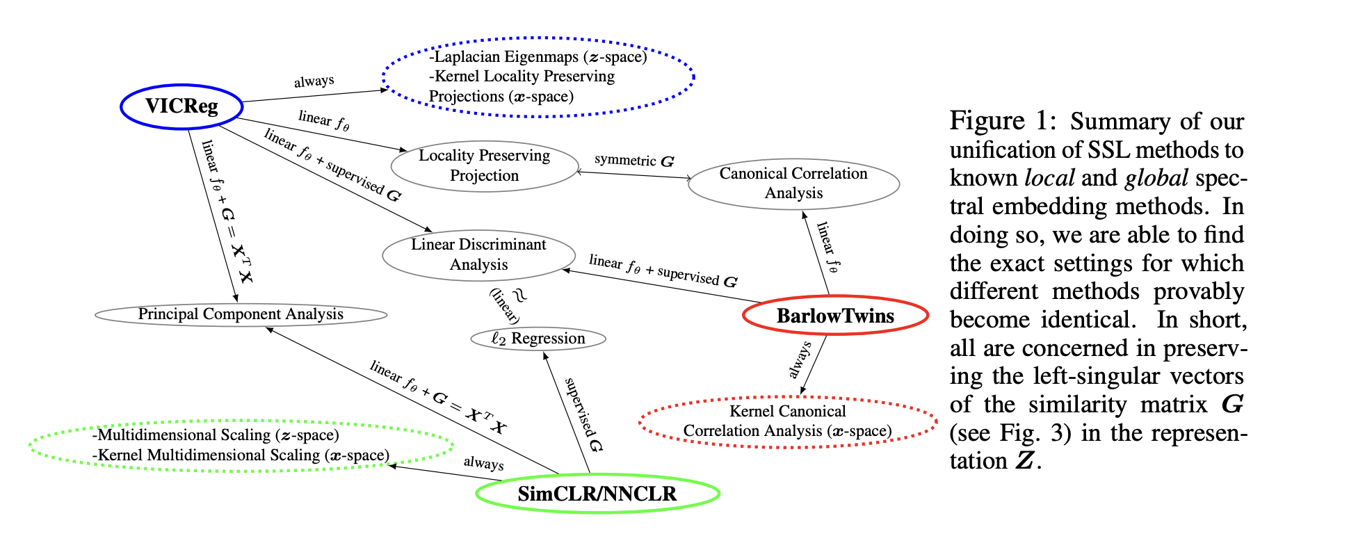
Interpretation as spectral clustering
A general study has been done in Contrastive and Non-Contrastive Self-Supervised Learning Recover Global and Local Spectral Embedding Methods
This paper considers a simplified model, when the views of the dataset are linear maps.
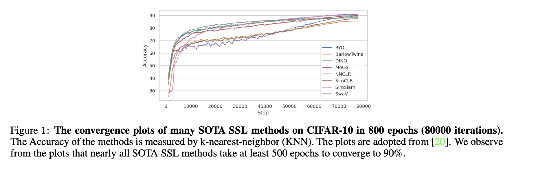
More efficient training for SSL models
Recent paper: EMP-SSL: TOWARDS SELF-SUPERVISED LEARNING IN ONE TRAINING EPOCH
claims that we can significantly speed-up training contrastive loss framework.
Originally, the methods are quite slow to train
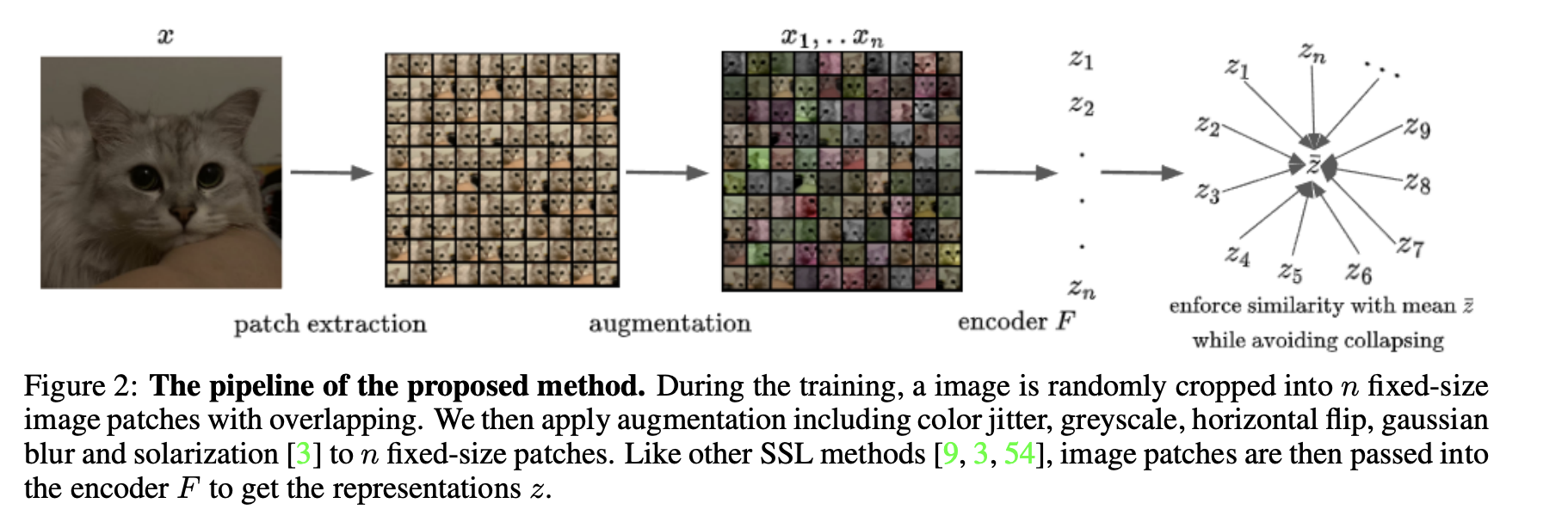
EMP-SSL
Idea is to split into really many patches!
Then, enforce similarity with the mean, simultaneously avoiding collapse.
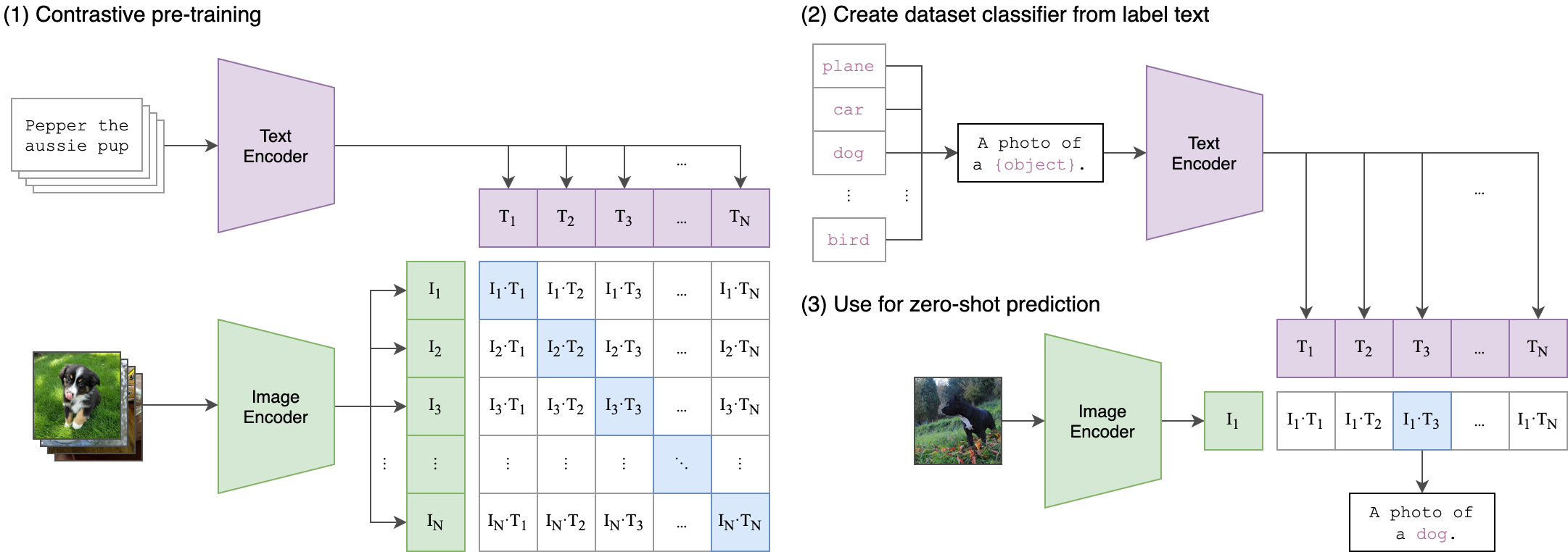
Contrastive learning for multimodal data
There is no much difference between contrastive learning for images and images/text.
The latter is even simpler, if the dataset is organized into pairs!.
This is the part of the famous CLIP model!
Some challenges for the CLIP model
The CLIP paper reports batch size 32k for training, i.e. the scaling $B^2$ for the model.
A good research question is wether we really need such a large batch size.
Some insights
- The type of data augmentation is very important
- Very large batch size (i.e., large number of negatives) is required for contrastive loss to work well.
- Typically, training is quite slow
Summary
- What is contrastive learning
- Popular losses
- SimCLR
- MoCo
- ByOL
- Barlow Twins
- VicReg
Next lecture: Few-shot learning/zero-shot learning/foundation models
- What is few-shot learning
- What is zero-shot learning
- Popular datasets for few-shot/zero learning
- Brief description of the concept of foundation models.