Lecture 11: One-shot/Zero-shot/Few-shot learning

Previous lecture: General tricks for efficient training:

• What is contrastive learning
• Popular losses
• SimCLR
• MoCo
• ByOL
• Barlow Twins
• VicReg

Current lecture: One-shot/Zero-shot/Few-shot learning

• What is few-shot learning
• Meta learning
• Main models and approaches (ProtoNets, SiameseNetworks, MAML)

What is few-shot learning

The few-shot learning (FSL) covers the case when we have very few samples for each class in the dataset.

When we’re talking about FSL, we usually mean $N$-way-$K$-Shot-classification.

$N$ stands for the number of classes, and $K$ for the number of samples from each class to train on.

Example applications

There are many cases:

• Face detection / identification
• Drug toxicity prediction
• Medical diagnosis: Few-shot learning can be used to diagnose medical conditions with limited data. The model can learn to recognize rare diseases with only a few examples
• Robotics

How to do few-shot learning

One can actually train a supervised learning classifier with enormous amount of classes.

I.e. a very strong baseline now is just to make a softmax loss for all classes in the training set.

The disadvantage is that we need quite a lot of memory for the linear layer.

Besides that, most of the few-shot learning approaches fall into the meta-learning area.

What is meta-learning?

Meta-learning (also known as learning to learn) learns sequentially:

Given a series of tasks, it improves the quality of predictions on new (unseen) tasks.

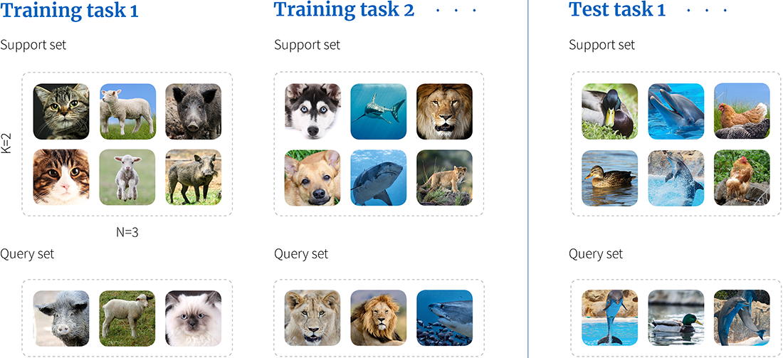
The Meta-learning framework involves training an algorithm using a series of tasks, where each task is a 3-way-2-shot classification problem consisting of a support set with three classes and two examples of each.

During training, the cost function evaluates the algorithm's performance on the query set for each task, given its respective support set.

At test time, a different set of tasks is used to assess the algorithm's performance on the query set, given its support set.

There is no overlap between the classes in the training tasks {cat, lamb, pig}, {dog, shark, lion},

and those in the test task {duck, dolphin, hen}.

As a result, the algorithm must learn to classify image classes generally rather than any particular set.

Support set and query set

Here, each task mimics the few-shot scenario, so for N-way-K-shot classification, each task includes $N$ classes with $K$ examples of each.

The task is specified by the support set (used for training) and query set (used for evaluation).

Meta-learning steps

At each step of the meta-learning, we update the model parameters based on a randomly selected training task.

The loss function measures some accuracy on the query set, based on the knowledge gained from the support set.

To evaluate the few-shot performance, we have to look at completely unseen tasks.

Main approaches to meta-learning

• Learning embeddings: We learn embeddings that tend to separate classes (note that this is similar to self-supervised learning in some sense, the difference is that we know few labels). Examples: Protonetworks, Siamese networks, Triplet networks, matching networks
• Prior knowledge about learning: We use prior knowledge to constrain the algorithm to choose parameters: MAML approach
• Prior knowledge about data: We use prior knowledge about the data: learn generative models from the data, generate new sample to augment

Pairwise comparisons

We can use ideas of self-supervised learning (strictly speaking, self-supervised learning ideas were motivated from few-shot learning, but in the course we are giving it vice-a-versa).

We can learn to distinguish between pairs (pairwise comparators) or we can learn to distringuish between many samples (multi-class comparators).

Two standard approaches with pairwise comparisons include:

• Siamese networks, 2015
• Triplet networks, 2016

Siamese network

In Siamese network, we take two shared networks. Given $x_a$ and $x_b$ they will output the probability that

$$\mathrm{Pr}(y_a = y_b)$$

using just binary cross-entropy loss (i.e. the output is passed through a sigmoid).

We randomly pick a pair.

This is not formally a N-way-K-shot task, but similar and can be adapted.

How we can adapt to such task?

Triplet network

In a triplet network, we (again) work with triplets $\{\mathbf{x}_{+},\mathbf{x}_{a},\mathbf{x}_{-}\}$, where the positive and anchor samples are from the same class, whereas the negative sample is from a different class.

The learning loss is the triplet loss with tries to push positive from negative up to a certain margin (look at the previous lecture).

Multi-class comparators

We can adapt pairwise comparators to the N-way-K-shot setting by assigning the class of the example of the query set to the maximally similar example in the support set.

Denote by $x_{nk}$ the support example number $k$ from with $n$-th class, and $y_{nk}$ the corresponding label.

Then, we can have:

• Matching Networks
• Prototypical Networks
• Relation Networks

Matching networks

Matching networks Vinyals et al. 2016 predict the one-hot encoded query-set label as a weighted sum of all of the one-hot encoded support-set labels $\{\mathbf{y}_{nk}\}_{n,k=1}^{NK}$.

The weight is based on computed similarity $a[\hat{\mathbf{x}},\mathbf{x}_{nk}]$ between the query $\hat{x}$ and all the training data $\{\mathbf{x}_{nk}\}_{n,k=1}^{N,K}$ \begin{equation}    \hat{\mathbf{y}} = \sum_{n=1}^{N}\sum_{k=1}^{K} a[\mathbf{x}_{nk},\hat{\mathbf{x}}]\mathbf{y}_{nk} \end{equation}

where the similarities have been constrained to be positive and sum to one. Motivated by attention mechanism!

To compute the similarity $a[\mathbf{x}_{nk},\hat{\mathbf{x}}]$ we pass $\mathbf{x}_{nk}$ through a network $f$, then $\hat{\mathbf{x}}$ through another network $g$,

then compute cosine similarity

\begin{equation} d[\mathbf{x}_{nk}, \hat{\mathbf{x}}] = \frac{\mbox{ f}[\mathbf{x}_{nk}]^{T}\mbox{ g}[\hat{\mathbf{x}}]} {||\mbox{ f}[\mathbf{x}_{nk}]||\cdot||\mbox{ g}[\hat{\mathbf{x}}]||}, \end{equation}

and normalize to probability as

\begin{equation} a[\hat{\mathbf{x}}_{nk},\mathbf{x}] = \frac{\exp[d[\mathbf{x}_{nk},\hat{\mathbf{x}}]]}{\sum_{n=1}^{N}\sum_{k=1}^{K}\exp[d[\mathbf{x}_{nk},\hat{\mathbf{x}}]]}. \end{equation}

The loss function is the entropy between ground truth and predicted labels.

Problems with matching networks

The main problem with matching network is when we have class imbalance (i.e., we depart from the N-way-K-shot scenario).

The algorithm is not robust to this case.

Prototypical networks

Prototypical networks Snell, 2017 are more robust to class imbalance and still used nowdays.

In this algorithm, the embeddings, corresponding to each class, are averaged to create a prototype.

The classification is done by selection of the closest prototype. They found that euclidean distance outperforms cosine distance.

$\displaystyle p_{\varphi}(y=k|x) = \frac{\exp(-d(f_{\varphi}(x), c_k))}{\sum_{k'=0}^{P-1}\exp(-d(f_{\varphi}(x), c_{k'}))}$, and we maximize the probability of the true class

Relation networks

Relation networks Santoro 2016 use the external memory idea (from the so-called relation module).

It has:

• Embedding
• Controller (typically, an LSTM to proces a sequence)
• An external memory module

At each step, the controller given the input $x_t$ (the images are shown sequentially to a module) and produces a key $k_t = f(x_t)$ which is either stored in a row of a matrix $M_t$ or used to retrieve a particular memory from $M_t$ based on the similarity:

$$ K(k_t, M_t(i)) = \frac{k_t \cdot M_t(i)}{\Vert k_t \Vert \Vert M_t(i) \Vert}. $$

The similarities are transformed into weights, the controller returns a weighted sum of $M_t(i)$.

A sophisticated rule for the update has been derived based on the number of usages.

]

Comparison of multiclass comparators

Model-agnostic meta-learning

Model-agnostic meta-learning

Takes the approach for general training in the meta-learning scenario: we have a sequence of tasks $\mathcal{T}_i$ and the model with parameters $\theta$.

The meta-objective to minimize in MAML is:

$\min_{\theta} \sum_{T_i \sim p(T)} L(T_i, f_{\theta_i}')$

where:

• $T_i$ is a task sampled from the distribution $p(T)$
• $L(T_i, f_{\theta_i}')$ is the loss on task $T_i$ after one or more gradient updates using the updated parameters $\theta_i' = \theta - \alpha \nabla_{\theta} L(T_i, f_{\theta})$

For optimization, we need to compute high-order gradients?

How to train you MAML

How to train your MAML paper improves working with MAML. The main reason is that the convergence of MAML training can be quite slow and erratic.

Issues:

1. Slow convergence
2. Second-order derivatives cost
3. Problems with Batch Normalization

MAML++

In MAML++ the update of the parameters is done after several gradients steps for a single task is done.

There are other tricks (engineering) that improve generalization

This improves generalization error on several datasets.

Reptile

The paper proposes Reptile algorithm as an alternative to MAML.

Input: Learning rate $\eta$, number of steps $k$, set of tasks $\mathcal{T}$, initial parameters $\phi$

Output: Updated parameters $\varphi$

1. for $iteration = 1, 2, ...$ do
2.   Sample task $\tau \in \mathcal{T}$, corresponding to loss $L_{\tau}$ on weight vectors $\phi$
3.   Compute $\tilde{\phi} = U_k^{\tau}(\phi)$, denoting $k$ steps of SGD or Adam
4.   Update $\phi \gets \varphi + \eta(\tilde{\phi} - \phi)$
5. end for

where $U_k^{\tau}(\phi)$ denotes $k$ steps of SGD or Adam on task $\tau$ starting from initial parameters $\phi$.

TADAM

Another influencial paper is TADAM: Task dependent adaptive metric for improved few-shot learning

Contributions:

• Introducing temperature into softmax scaling of prototype networks
• Use the mean of the class prototypes as the task representation and put them into conditional batch normalization.

Simple baseline for few-shot classification

A BASELINE FOR FEW-SHOT IMAGE CLASSIFICATION proposes a very simple baseline for few-shot classification which is often difficult to beat in terms of generalization accuracy in practice.

It also critizes the evaluation protocol: people use different training sets, different architectures, making it difficult to find the actual reason for the accuracy improvement.

Baseline works as follows:

• We pretrain using cross-entropy loss in the supervised way with softmax (main challenge: very large softmax layer).

How to modify for new (unseen) classes?

Reptile

The paper propose a Reptile algorithm as an alternative to MAML

Simple baseline: unseen classes

If we get a new class with several examples, we can process it with the backbone network and then compute the prototypes by averaging.

Datasets

The methods for few-shot learning are typically tested on

• Omniglot (analogue of MNIST)
• MiniImageNet (subclass of ImageNet with 100 classes with 600 examples each)
• Caltech-UCSD Birds

Current State-of-the art (SOTA)

The current SOTA for 5-way Miniimagenet can be found here

Current (as of April 18, 2023) record

Current record is described in the paper Pushing the Limits of Simple Pipelines for Few-Shot Learning: External Data and Fine-Tuning Make a Difference.

P > M > F pipeline

1. Pretrain on large supervised tasks
2. Meta-learning using protonet
3. (Interesting idea): fine-tuning with random augmentation on the test task (actually helps!)

Few-shot learning in NLP

We can also extend the problem statement of few-shot learning (or meta-learning) to the NLP domain.

Large language models do have very interesting properties!

Language models are few-shot learners

GPT-3 paper empirically shows that GPT-3 models work well as few-shot learners.

The idea is that we can use a pretrained GPT model by putting some (context) examples at the top.

Does it really learn new concepts?

Citation from the paper:

In the context of language models this has sometimes been called “zero-shot transfer”, but this term is potentially ambiguous: the method is “zero-shot” in the sense that no gradient updates are performed, but it often involves providing inference-time demonstrations to the model, so is not truly learning from zero examples. To avoid this confusion, we use the term “meta-learning” to capture the inner-loop / outer-loop structure of the general method, and the term “in context-learning” to refer to the inner loop of meta-learning. We further specialize the description to “zero-shot”, “one-shot”, or “few-shot” depending on how many demonstrations are provided at inference time. These terms are intended to remain agnostic on the question of whether the model learns new tasks from scratch at inference time or simply recognizes patterns seen during training – this is an important issue which we discuss later in the paper, but “meta-learning” is intended to encompass both possibilities, and simply describes the inner-outer loop structure<

Zero-shot learning

In Zero-Shot Learning, the data consists of the following:

• Seen Classes: These are the data classes that have been used to train the deep learning model.
• Unseen Classes: These are the data classes on which the existing deep model needs to generalize. Data from these classes were not used during training.
• Auxiliary Information: Since no labeled instances belonging to the unseen classes are available, some auxiliary information is necessary to solve the Zero-Shot Learning problem. Such auxiliary information should contain information about all of the unseen classes, which can be descriptions, semantic information, or word embeddings.

In Zero-shot learning, we have description of the classes given.

Not too many agreed benchmarks for it.

Classical tasks include image tagging.

Now we can use CLIP models for it.

Summary

• What is few-shot learning
• Meta learning
• Main models and approaches (ProtoNets, SiameseNetworks, MAML)

Next lecture: Adversarial attacks, adversarial training, robustness

• Adversarial attacks
• Adversarial training
• Robustness of DL models (using randomized smoothing)