Lecture 12: Adversarial attacks and training

Previous lecture: Few-shot learning

• What is few-shot learning
• Meta learning
• Main models and approaches (ProtoNets, SiameseNetworks, MAML)

Current lecture: Adversarial attacks and training

• Adversarial attacks
• Adversarial training
• Robustness of DL models (using randomized smoothing)

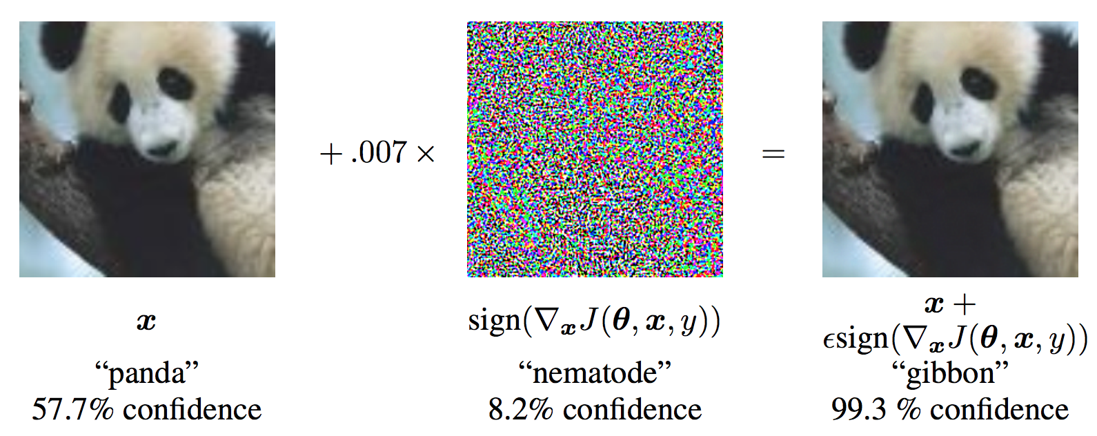
Adversarial attacks: how they were developed.

Ian Goodfellow looked at the multiclass classifier, given by the model $p(c \vert x),$ (probability of the class condition at the input).

Suppose we want to move smoothly from one class (cat) to another class (dog).

So, you can just maximize the probability of the image of being a dog, moving in the direction of the gradient

$$\nabla \log p(c_2 \vert x), $$

But they found an extremely suprising result: even small modification leads to large missclassification.

Problem statement

White-box small-norm attack on a deep neural network model is the following optimization task.

Let $p(x) \in \mathbb{R}^c$ be the classifier with $c$ classes. Then the minimal norm attack is defined as the

solution to the following optimization problem:

$$\min \Vert \varepsilon \Vert\, \mbox{s.t. } \arg \max p(x + \varepsilon) \ne \arg \max p(x)$$

I.e. the minimal-norm perturbation that changes the class.

Existing models are notoriously unstable!

Different types of attacks

There are different types of adversarial attacks (whitebox, greybox, blackbox).

The can be universal or not. They can be one-shot and iterative.

Whitebox attacks

In whitebox attacks we know the weights of the model (which is not always the case).

The most well-known attacks are:

1. Fast Gradient Sign Method (FGSM): This attack involves adding a small perturbation to the input image by computing the gradient of the loss function with respect to the input.

2. Projected Gradient Descent (PGD): This attack is an iterative version of FGSM, where the perturbation is added in small steps until a certain threshold is reached.

3. DeepFool: This attack finds the minimum distance from the input image to the decision boundary of the classifier and then adds a small perturbation in that direction.

4. Carlini-Wagner (CW) Attack: This attack is designed to minimize the distance between the original image and the adversarial image while also ensuring that the adversarial image is misclassified.

5. Universal Adversarial Perturbation (UAP): This attack generates a single perturbation that can be added to any input image to cause misclassification.

Fast sign gradient method

Fast Gradient Sign Method (FGSM) is a popular whitebox adversarial attack that involves adding a small perturbation to the input image by computing the gradient of the loss function with respect to the input. Mathematically, the FGSM attack can be expressed as:

$$ \hat{x} = x + \epsilon \cdot \mathrm{sign}(\nabla_{x} p(y \vert x)) $$

where $\text{adv}{x}$ is the adversarial image, $x$ is the original image, $\epsilon$ is the magnitude of the perturbation, $p(x, y)$ is the loss function, input image $x$, and true label $y$, and $\nabla{x}$ is the gradient operator with respect to $x$. The sign function is used to ensure that the perturbation is added in the direction that maximizes the loss function.

The derivation of FGSM is done by linearizing the loss function and solving the norm-constrained problem!

It does not necessary gives the optimal solution.

PGD attack

Projected Gradient Descent (PGD) is a more powerful whitebox adversarial attack that iteratively applies the FGSM attack with a small step size and then projects the resulting perturbed image back onto the attack set.

Mathematically, the PGD attack can be expressed as:

$$ x_0 = x, \quad x_{t+1} = \text{Clip}(x_t + \alpha \cdot \text{sign}(\nabla_{x} p(y \vert x_t)) $$

PGD is more effective, but computationally more expensive as well.

Carlini-Wagner attack

The Carlini-Wagner (CW) attack is a state-of-the-art whitebox adversarial attack that is designed to be more effective than PGD against defenses that use gradient masking or gradient obfuscation techniques. The CW attack formulates the problem of finding an adversarial perturbation as an optimization problem that minimizes the distance between the original image and the perturbed image, subject to a constraint on the classification loss.

Mathematically, the CW attack can be expressed as:

$$ \min_{\delta} \Vert \delta \Vert_{p} + c \cdot f(x+\delta, y) $$

where $\delta$ is the adversarial perturbation, $\Vert \cdot \Vert{p}$ is a norm function, $c$ is a hyperparameter that controls the trade-off between the distance and the loss term, and $f(\cdot, y)$ is a function that measures the classification loss of the perturbed image with respect to the target class $y$.

DeepFool

DeepFool attack uses the idea of linearized decision boundary.

Suppose we have a binary classifier, and the separation function is given as $f(x) = 0$.

$f(x) > 0$ corresponds to one class, $f(x) < 0$ to another.

The best attack would be given by the closest point to the boundary.

To find such point, we linearize the function as

$$f(x) \approx f(x_0) + f'(x), x - x_0.$$

Finding the closest point to the boundary can be done analytically.

Then we can update iteratively

Initialize: $x := x_0$

Iteration: $r_i := -\frac{f(x_i) \nabla f(x_i)}{\Vert \nabla f(x_i) \Vert^2}$, $x_{i+1} = x_i + r_i$.

Universal adversarial attacks

Idea of universal adversarial attacks has been proposed in the paper

The idea is to have a single image such that adding it to all images fools the classifier.

Universal adversarial attacks: algorithms

Original idea of constructing universal adversarial attacks uses geometrical ideas

UAP: numbers and how they look like

Typical numbers are 60-80% of fooling!

Black-box attacks

In the black-box attacks we only have limited knowledge about the target model, i.e.

1. We don't know the weights
2. We only have access to logits or even predictions of the model.

How we can construct such kind of attacks?

Some types of black-box attacks

Transfer attacks:

In this attack, the attacker trains a substitute model to mimic the behavior of the target model using only input-output pairs. The substitute model can then be used to generate adversarial examples that can fool the target model.

Query-based attacks: In this attack, the attacker submits a large number of input queries to the target model to infer its internal behavior. This information can then be used to generate adversarial examples.

Zeroth-order optimization: In this attack, the attacker uses only the output of the target model to generate adversarial examples, without any knowledge of the internal parameters or architecture of the model.

Example black-box attacks

One of the simplest and efficient black-box attacks is Square attack

We find squares by random search.

The squares are sampled randomly according to some distributions.

Beyond small-norm attacks

Small-norm attacks are done in the digital domain. But small-norm is not always the right attack model.

Important classes of attacks include:

• Sparse attacks
• Patches
• Semantic transformations (rotations, gaussian blurring, etc.)

Surprisingly, most of them break the classifiers!

Real-world attacks

A significant attention has been given to real-world attacks.

How to build real-world attacks

Building real-world attacks is an interesting engineering task.

Since the neural networks are unstable with respect to small perturbations, they also get really well back

if the noising process is put back in place.

I.e., when you print and you take the photo, the image is distorted and it can no longer by an adversarial example.

Attacking in real world

The first paper is Adversarial examples in the physical world by Alexey Kurakin, Ian Goodfellow, Samy Bengio

Idea was super-simple: incorporate image transformations (rotations/blur/brightness) into the process of generating attacks.

The attacks should be attacks under all of those transformations.

At later paper the approach called (expectations over transformations) has been proposed.

Instead of using $f(x)$, they used

$$\hat{f}(x) = E_T T(f(x))$$

as the loss function.

Other approaches include synthetic data generation, mapping real-life photos using generative adversarial networks (GANs), etc.

Defending against attacks

Adversarial attacks pose significant danger in several scenarios, thus it is important to develop defenses.

The defenses can be empirical or certified. Certified means that we guarantee that for a fixed attack model, the prediction will not change. We can do certain certification for small-norm attacks.

Emprical defenses make certain modifications to the training or inference procedures.

Empirical defenses against adversarial attacks

There are several standard approaches against attacks. Among them:

1. Adversarial training: This involves training the model on both clean and adversarial examples to improve its robustness against attacks.
2. Defensive distillation: This involves training the model to output softened probabilities instead of hard probabilities, which can make it more difficult for attackers to generate adversarial examples.
3. Randomization: This involves adding random noise or perturbations to the input or model parameters to make it more difficult for attackers to generate adversarial example
4. Gradient masking: This involves hiding the gradient information from attackers by adding noise to the gradients or using gradient obfuscation techniques.
5. Ensemble methods: This involves combining multiple models to improve their robustness against attacks. Adversarial examples that fool one model may not fool another, making it more difficult for attackers to succeed.

Adversarial training

In adversarial training, we aim at minimizing the loss at the worst possible sample in the vicinity of the current one.

\begin{equation} \min_{\theta} \mathbb{E}_{x,y \sim p_{data}(x,y)} [\max_{\delta \in S} \mathcal{L}(f_{\theta}(x+\delta), y)] \end{equation}

The solution of the inner maximization problem is done by several PGD steps, giving much slower training time, but increased robustness.

The idea of adversarial training has been proposed in the paper by Madry et. al

Adversarial training for free

Adversarial training for free proposes two things:

1. Compute the gradient with respect to the input and parameters on the same step;
2. Train on the same mini-batch $m$ times (to mimic $m$-step PGD attacks).

Leads to neglible overhead!

Fast is better than free

Next step is Fast is better than free paper, which proposes the following idea.

In 'Adversarial training for free' perturbation from the previous sample is used as an initialization for the next sample.

It is difficult to believe that it is a good starting point, but it is non-zero.

Instead, the authors initialize the perturbation at random, and use 1 step of FGSM in training.

Smooth adversarial training

Smooth adversarial training

Simple idea in the Quoc Le style: replace ReLU (non-smooth) with its smooth variant, significantly improves robustness.

Randomized smoothing

Let $f(x)$ be our binary classifier. Existence of attacks means that under a small perturbation $f(x + \varepsilon)$ changes a lot. Thus, it means that $f(x)$ should have large Lipschitz constant.

One can try to make the classifier smoother by imposing certain normalization techniques, such as spectral normalization (which is typically a bounded norm of the linear layer).

An alternative approach is to modify the inference procedure by smoothing over small perturbation.

It is called randomized smoothing.

Randomized smoothing: Theory

Randomized smoothing has been proposed by Cohen et. al

The idea is to replace the inference procedure with smoothing

$$\hat{f}(x) = E_{\varepsilon \sim N(0, \sigma^2)}f(x + \varepsilon).$$

The Cohen paper uses the indicator function under smoothing.

It is basically a voting method: we sample attacks, and select the class that is predicted the most times.

Certified radius bound

Let $p_A$ and $p_B$ be the probability of true class and false class from the randomized classifier.

We can not evaluate them directly, therefore we can get access to their bounds $\underline{p_A}$ and $\overline{p_B}$.

Then, the smoothed classifier is guaranteed to get the same prediction for an $x$ within the radius

$$R = \frac{\sigma}{2}\left(\Phi^{-1}(\underline{p_A}) - \Phi^{-1}(\overline{p_B})\right),$$

where $\Phi^{-1}$ is an error function.

Randomized smoothing: Theory

A more complicated estimate for the Randomized Smoothing has been obtained by Salman et. al.

Let $f(x)$ be the base classified, $f(x) \in [0, 1]$. Let $\hat{f}(x)$ be a smoothed classified with $\sigma=1$.

Let $\Phi(x)$ be the error function.

Then,

$$g(x) = \Phi^{-1}(\hat{f})$$

has Lipschitz constant one.

Randomized smoothing: discussion

We have

1. Vanilla accuracy (of the base classifier)
2. Accuracy of the smoother classifier
3. Certified accuracy (vs. the attack radius).

If we train the base classifier only, the smoothed accuracy will be smaller.

In practice, we can add maximize the accuracy of the smoothed classified, by minimizing

$$L(\hat{f}) \rightarrow \min.$$

Note, that during training we can replace smoothing just by random Gaussian augmentation.

This will give an unbiased estimate of the gradient.

How we measure robustness of deep learning model

A standard protocol to measure robustness of deep learning models is to attack them using PGD attacks.

A standard benchmark is RobustBench

Lets have a look at the leaderboard: https://robustbench.github.io/

Summary

• Adversarial attacks
• Adversarial training
• Robustness of DL models (using randomized smoothing)

Next lecture: Generative models I

• Autoregressive models
• Variational Autoencoders