Lecture 13: Generative models I

Previous lecture: Adversarial attacks and training

• Adversarial attacks
• Adversarial training
• Robustness of DL models (using randomized smoothing)

Current lecture: Generative models I

• Autoregressive models
• Variational Autoencoders

Generative models

So far, we talked about supervised learning and self-supervised learning, where the goal is to encode an object $x$

into a meaningful feature representation $E(x)$ such that we can distinguish different object.

The goal of generative models is different:

Given samples $x_1, \ldots, x_N$ from the unknown probability distribution $p(x)$, we want to learn the probability distribution itself.

The minimum what we want to learn is a model that allows to sample from the distribution itself.

In some cases, we can also learn the density $p(x)$, so we can evaluate the log-likelihood itself.

We have encountered generative models when we talked about transformer models.

GPT is a generative autoregressive model.

Types of generative models

Today, there are quite a lot generative models.

Historically, one of the first family for generative models were autoregressive models, that focus on predicting sequence values in the future.

Other important directions which we will cover in this course include:

• Generative adversarial networks (implicit generative models)
• Variational autoencoders
• Diffusion models

They are very different concepts, but they all solve the problem of learning (parametric form) of high-dimensional probability distribution from samples.

Probabilistic autoregressive model

The autoregressive model is based on the representation of the probability density (for the continuous density) or probability (for discrete symbols as)

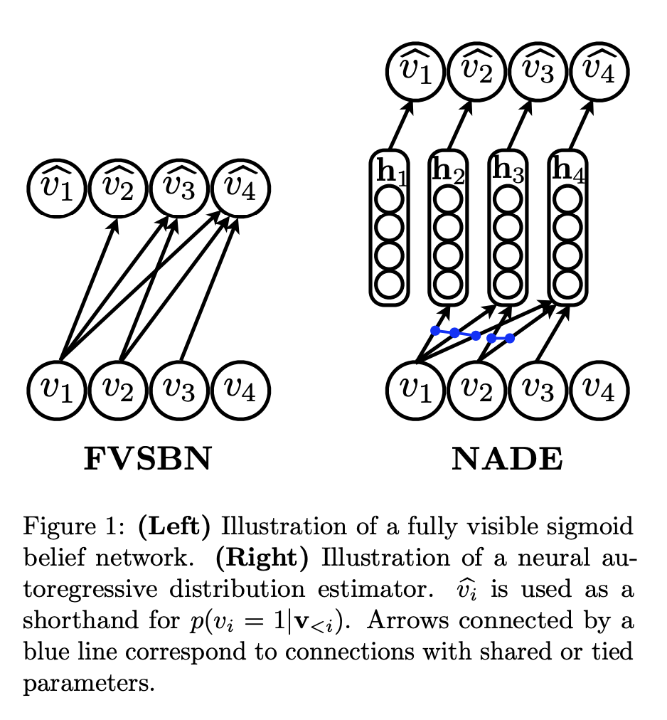
$$p(x_1, \ldots, x_T) = \prod_{t=1}^T p(x_t \vert x_{t-1}, \ldots, x_1).$$

NADe

The first neural autoregressive distribution estimator has been proposed in The Neural Autoregressive Distribution Estimator in 2011

The architecture is not up-to-date, but quite instructive. It was motivated by fully visible sigmoid belief network, proposed as early as 1992! In FVSBN, the value is conditioned to the previous ones using 1-layer network.

PixelCNN

The idea of variational like-lihood based model for images have been proposed in two papers:

Conditional image generation with PixelCNN decoders

Pixel Recurrent Neural Networks

Images formally is not a sequence, so we need to define a certain order.

PixelCNN ordering

In PixelCNN , the conditional distribution is modelled using convolutional neural network.

There are several variants to model such conditional distributions.

PixelRNN paper uses LSTM to build such conditional distribution.

In Conditional image generation with PixelCNN decoders the ReLU units are replaced with masked gated convolutions:

$$y = \operatorname{tanh}W_{k, f} * x) \odot \sigma(W_{k, g} * x).$$

It uses the raster scan with the following mask on the filter!

In also uses two blocks to increase the receptive field: vertical and horizontal. One conditions only on the current row, the second conditions on all the previous rows.

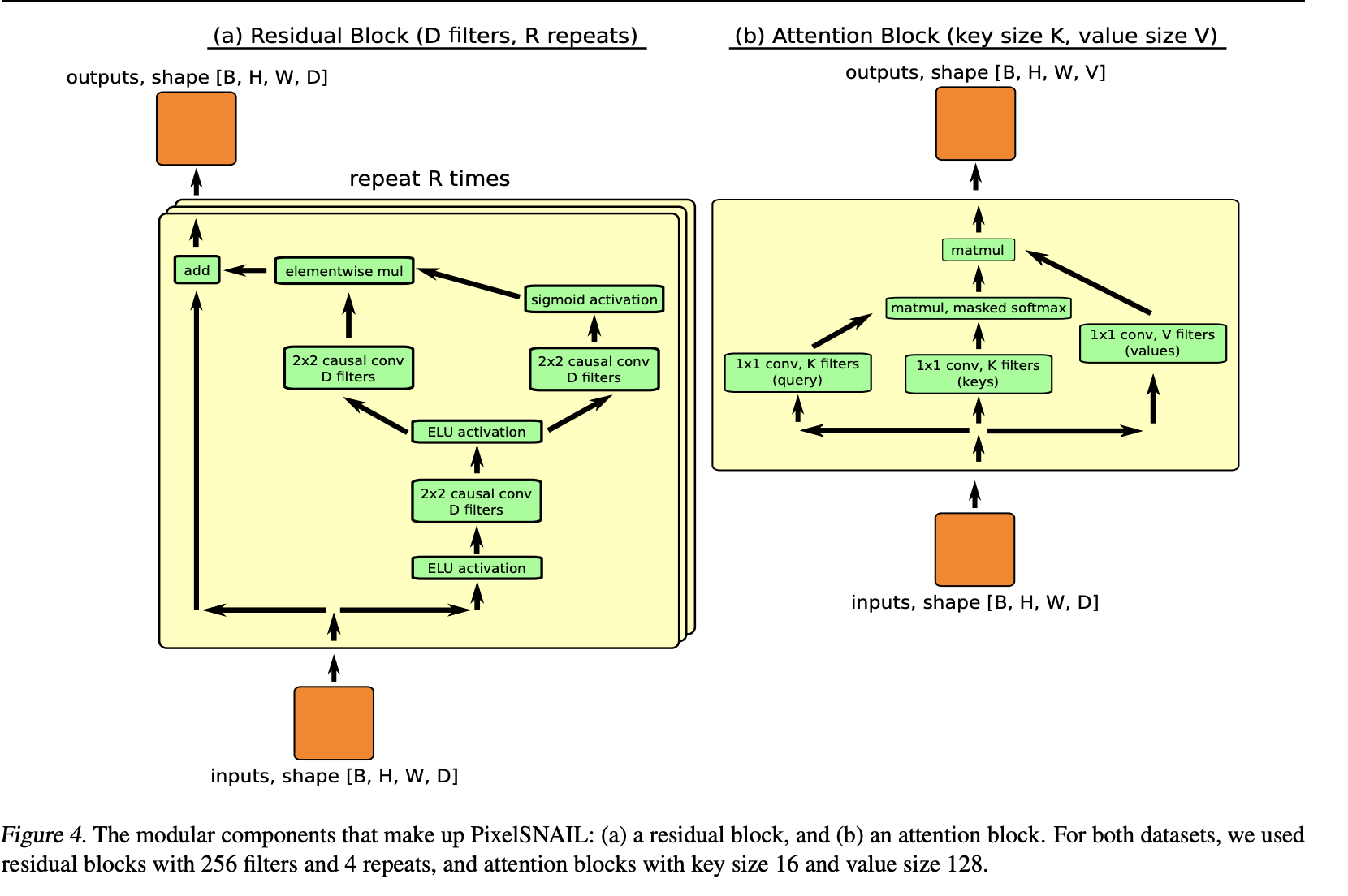
Improving PixelCNN

Certain improvents have been proposed in the paper Xi Chen, Nikhil Mishra, Mostafa Rohaninejad, and Pieter Abbeel. PixelSNAIL: An Improved Autoregressive Generative Model

The available options to model conditional distributions:

1. Traditional RNNs, difficult to model long-range dependence for images
2. Masked (gated) convolutions
3. Of couse, we can use self-attention!

PixelSNAIL architecture

The whole decoder architecture has the following form:

PixelSNAIL-blocks

The blocks mentioned in the previous slide have the following form.

Applications of autoregressive generative models

The autoregressive generative models have been proposed for images, but the biggest usage and success have been achieved not for image, but for time-series (which is natural).

For audio signals and tasks, such models held state-of-the art for quite a long time and still are being used.

Namely, this is the WaveNet architecture.

WaveNet

In Generative model for raw audio the WaveNet architecture has been proposed.

Similarly to PixelCNNs (van den Oord et al., 2016a;b), the conditional probability distribution is modelled by a stack of convolutional layers. There are no pooling layers in the network, and the output of the model has the same time dimensionality as the input. The model outputs a categorical distribution over the next value xt with a softmax layer and it is optimized to maximize the loglikelihood of the data w.r.t. the parameters. Because log-likelihoods are tractable, we tune hyperparameters on a validation set and can easily measure if the model is overfitting or underfitting.

Causal convolutions

The model can not depend on future timesteps, i.e. be causal.

For images, the analogue of the causal convolution is masked convolution, where in the convolution the 'wrong' pixels are multiplied to zero.

At training, such convolutions can be done simultaneously, whereas at inference we have to do prediction one at a time.

Q: What is the difference to recurrent neural networks (RNN)?

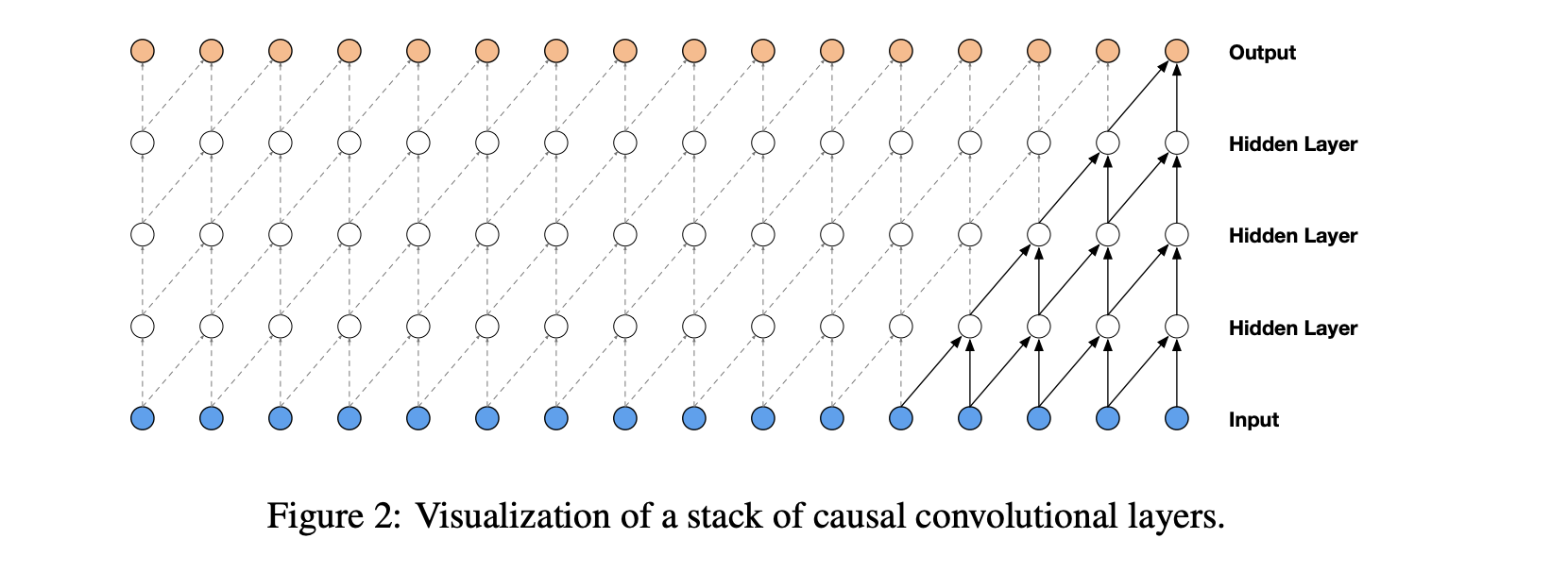
Properties of causal convolutions

• They are faster to train than recurrent neural networks, especially for longer sequences
• For longer sequence we need more hidden layers: the number of hidden layers determine the receptive field of the model.

Dilated causal convolutions

• A dilated convolution (also called a trous ` , or convolution with holes) is a convolution where the

filter is applied over an area larger than its length by skipping input values with a certain step. It is equivalent to a convolution with a larger filter derived from the original filter by dilating it with zeros, but is significantly more efficient

• Stacked dilated convolutions enable networks to have very large receptive fields with just a few layers, while preserving the input resolution throughout the network as well as computational efficiency.

• The dilation is doubled every layer

Architecture details

The model in the non-linearity uses gated units of the form

$$\mathbf{z}=\tanh \left(W_{f, k} * \mathbf{x}\right) \odot \sigma\left(W_{g, k} * \mathbf{x}\right)$$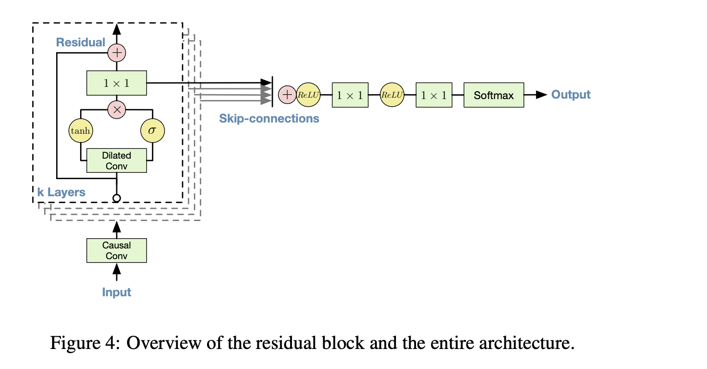

Generating speech with Wavenet (conditioning)

WaveNet architecture has been used for Text-to-Speech generation.

In order to condition the generation on text, the conditioning has been introduced into the architecture.

It is achieved by upsampling such local features to the level and using inside the gating mechanism

Given $h_t$, possibly with a lower sampling frequency than the audio signal, e.g. linguistic features in a Text-to-Speech (TTS) model.

This time series is first transformed using a transposed convolutional network (learned upsampling) that maps it to a new time series $\mathbf{y}=f(\mathbf{h})$ with the same resolution as the audio signal, which is then used in the activation unit as follows:

$$ \mathbf{z}=\tanh \left(W_{f, k} * \mathbf{x}+V_{f, k} * \mathbf{y}\right) \odot \sigma\left(W_{g, k} * \mathbf{x}+V_{g, k} * \mathbf{y}\right) $$

Note the gating mechanism again (actually, quite powerful idea).

Summary for simple autoregressive models

• Autoregressive models follow the same ideology as modern transformers (modelling conditional distributions)
• First attempts included RNN/GRU type model for the conditional distributions
• PixelCNN has reached good results (at that time) for modelling image distribution at the pixel level. It used masked convolutions
• WaveNet has got SOTA (at that time) for generation of speech from text, music and audio. It uses dilated causal convolutions.
• Generation is very slow due to generation by one sample at a time.

The autoregressive models represent the probability in a tractable manner.

The variational autoencoders (VAE) represent probability in a way that likelihood can not be computed, but can be optimized using variational inference and samples.

But first, we will discuss models based on the transformations of the random variable.

Other models

The autoregressive models can be considered as a special case of a more general construction:

Learning an invertible transformation from a simple distribution with a tractable Jacobian.

There are several examples of such approach: Real NVP, Glow.

Lets discuss the idea

Change of variables formula

The idea of real NVP is to parametrize the distribution as:

$$z \sim p(z), x = f^{-1}(z) \quad \mbox{(generation)},$$

where $f$ is a parametrized invertible transformation.

The change of variables formula gives $$p_X(x)=p_Z(z)\left|\operatorname{det}\left(\frac{\partial g(z)}{\partial z^T}\right)\right|^{-1}$$

Parametrizing the mapping

In RealNVP model, $f$ is parametrized as a superposition of affine coupling layers of the form $$ \begin{aligned} y_{1: d} & =x_{1: d} \\ y_{d+1: D} & =x_{d+1: D} \odot \exp \left(s\left(x_{1: d}\right)\right)+t\left(x_{1: d}\right) \end{aligned} $$

The Jacobian of such kind of mapping is triangular, and the determinant (and its logarithm) is easily computed.

Glow

In Glow model

Invertible $1 \times 1$ convolutions are added into the architecture.

Later development

• The formulas for change of variables are used in diffusion models
• They are also used in FFJord approaches, when the forward model is parametrized by a Neural Ordinary Differential Equation.

Now, lets get to the variational autoencoders!

Variational autoencoders

Now we will discuss VAE, which is one of the most interesting and powerful class of generative models.

VAE has been introduced in Autoencoder Variational Bayes and

in the paper and has become one of the most influencial approaches in generative models.

Several reviews are available, for example this one.

Standard autoencoder

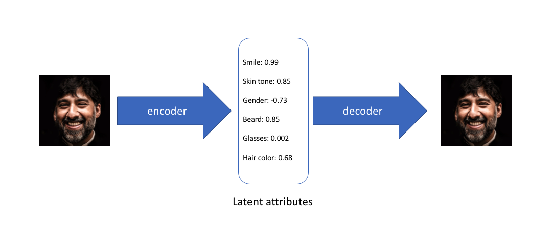
VAE intuition

We did not discuss too much classical autoencoder: we want to map an input $x$ to the latent space and then map back in order to reconstruct the initial image.

Problems:

• In the latent space we can just 'remember' the input
• Such model can not generate new samples

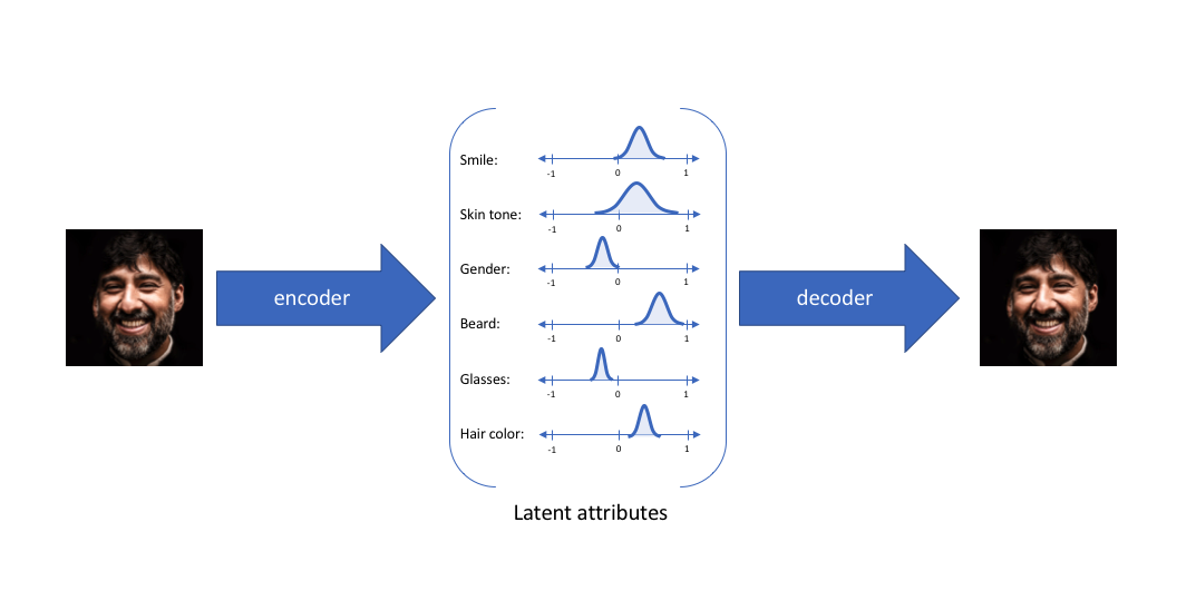
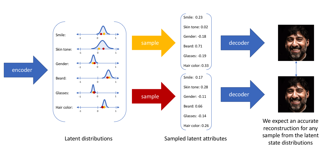
VAE intuition (2)

In VAE, we learn not the exact features, but some intervals (distributions of them).

I.e., the encoder maps the input into a certain distribution (which can be, of course, close to a delta-function).

Now, lets come up with a mathematical formalism.

The model

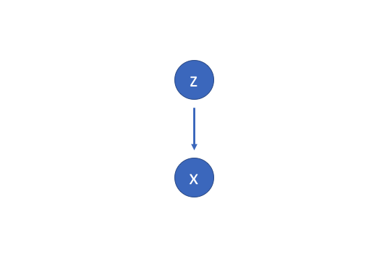
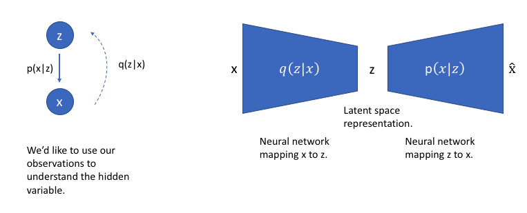
Suppose there exists a hidden variable $z$ that generates the output variable $x$.

We know the distribution of $z$, $p(z)$, we know the distribution of $x$ conditioned to $z$, $p(x \vert z)$.

If we want to encode, we need to know the distribution $p(z \vert x)$. This can be done by using Bayes formula:

$$p(z \vert x) = \frac{p(x \vert z) p(z)}{p(x)}, \quad p(x) = \int p(x \vert z) p(z) dz. $$

$p(x)$ is very difficult to evaluate in the general case!

Approximating the distribution

$$p(z \vert x) = \frac{p(x \vert z) p(z)}{p(x)}, \quad p(x) = \int p(x \vert z) p(z) dz. $$

We can use variational inference!

Lets approximate $p(z \vert x)$ by another distribution $q(z \vert x)$

Now we can minimize the distance $\min \mathrm{KL}\left( {q\left( {z|x} \right)||p\left( {z|x} \right)} \right)$, where $\mathrm{KL}$ is the Kullback–Leibler divergence between to distributions.

KL-divergence

KL-divergence between two continuous distributions is defined as

$$\mathrm{KL}(p || q) = E_p \log \frac{p}{q} = \int p(x) \log \frac{p}{q}$$

KL is a metric between two distributions, it has the following properties:

1. $\mathrm{KL}(p || q) \geq 0$
2. Is non-symmetric
3. If it is zero, the distributions are the same.

Deriving VAEs formulas

Recall, that we are minimizing $\min \mathrm{KL}\left( {q\left( {z|x} \right)||p\left( {z|x} \right)} \right)$ over $q$.

\begin{aligned} \mathrm{KL}[\mathrm{q}(\mathrm{z}) \| \mathrm{p}(\mathrm{z} \mid \mathrm{x})] & =\int_z \mathrm{q}(\mathrm{z}) \log \frac{\mathrm{q}(\mathrm{z})}{\mathrm{p}(\mathrm{z} \mid \mathrm{x})} \\ & =-\int_z \mathrm{q}(\mathrm{z}) \log \frac{\mathrm{p}(\mathrm{z} \mid \mathrm{x})}{\mathrm{q}(\mathrm{z})} \\ & =-\left(\int_z \mathrm{q}(\mathrm{z}) \log \frac{\mathrm{p}(\mathrm{x}, \mathrm{z})}{\mathrm{q}(\mathrm{z})}-\int_{\mathrm{z}} \mathrm{q}(\mathrm{z}) \log \mathrm{p}(\mathrm{x})\right) \\ & =-\int_z \mathrm{q}(\mathrm{z}) \log \frac{\mathrm{p}(\mathrm{x}, \mathrm{z})}{\mathrm{q}(\mathrm{z})}+\log \mathrm{p}(\mathrm{x}) \int_z \mathrm{q}(\mathrm{z}) \\ & =-\mathrm{L}+\log \mathrm{p}(\mathrm{x}) \end{aligned}

The value $L$ is called variational lower bound.

We get

$$L = \log p(x) - \mathrm{KL}(\mathrm{q}(\mathrm{z}) \| \mathrm{p}(\mathrm{z} \mid \mathrm{x}))$$

Since KL-divergence is non-negative, we get

$$\log p(x) \geq L.$$

Also, since for a fixed $x$ $\log p(x)$ is a constant, minimizing over $q = q(z \vert x)$ of the original KL divergence is equivalent to the maximization of $L$.

ELBO

This bound is typically referred to as ELBO (Evidence Lower Bound).

We have (recall that $p(x, z) = p(x \vert z) p(z)$,

$$L = \int_z q(z) \log \frac{p(x, z)}{q(z)} = {E_{q\left( {z|x} \right)}}\log p\left( {x|z} \right) - KL\left( {q\left( {z|x} \right)||p\left( z \right)} \right) $$

These two terms have clear interpretation.

The first term is a reconstruction term of the output from the latent vector.

The second term is the similarity of the the distribution of $q(z \vert x)$ to a prior distribution $p(z)$.

Using ELBO

We can use $q(z \vert x)$ as the encoder in the architecture to infer possible latent variables $z$ for a given $x$.

We can parametrize $q(z \vert x)$ by a neural network.

But what actually this neural network will output?

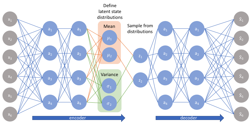
Parametrizing the latent distribution as Gaussians

The classical VAE parametrizes the latent distribution $q(z \vert x)$ as a Gaussian with mean value $\mu$ and diagonal covariance matrix $\sigma$.

The neural network will predict $\mu_j$ and $\sigma_j$ for each latent variable.

$\sigma_j$ has to be non-negative, so typically $\log \sigma_j$ is predicted rather than $\sigma_j$ itself.

But, the computational graph is stochastic.

How we differentiate through it?

But before...

Before it is needed to mention that the KL-divergence between two Gaussian can be computed analytically.

The decoder network $p(x \vert z)$ will also produce mean value and variance for each pixel!

So:

1. We pass $x$ though a network to get $\mu_{z \vert x}, \sigma_{z\vert x}$
2. Evaluate KL-divergence between $N(\mu_z, \sigma_z)$ and $p(z)$
3. We sample from this distribution
4. Using decoder network, predict $\mu_{x \vert z}$ and $\sigma_{x \vert z}$ for those samples
5. Evaluate the log-likelihood of the original input $x$.

How we compute the gradients?

ELBO has the following form:

$$L = {E_{q\left( {z|x} \right)}}\log p\left( {x|z} \right) - KL\left( {q\left( {z|x} \right)||p\left( z \right)} \right)$$

We need to compute the gradient with respect to the parametres of $p(x \vert z)$ and parameters of the distribution $q$ (also called variational parameters).

The main challenge is the first terms, since for Gaussians the second term is an analytic formula.

Gradient of $E_{q\left( {z|x} \right)}\log p\left( {x|z} \right)$ with respect to $p$ can be computed as an expectation:

$$ \nabla_p E_{q\left( {z|x} \right)}\log p\left( {x|z} \right) = E_{q\left( {z|x} \right)} \nabla \log p\left( {x|z} \right)$$

The gradient with respect to the varitional parameters $q$ is much trickier.

Fortunately, for basic distributions the expectation over parameter-dependent distribution can be estimated using reparametrization trick.

Reparametrization trick

For VAEs, a special technique called reparametrization trick has been proposed.

For Gaussians, the trick is simple.

1. Sample $\varepsilon$ from $N(0, 1)$.
2. Output $\mu + \sigma \varepsilon$.

Now we can differentiate with respect to $\sigma$ and $\varepsilon$.

In general, when we have losses of the form

$E_{z \sim q} h(q)$ it is not so easy to compute their gradient efficiently.

You can do quite

Estimating the likelihood in VAEs

Once the model is trained, we can:

• Generate samples from it
• Do encoding of the input to the latent space
• We can also estimate the likelihood of the model by using importance sampling technique.

$$ \log p_{\boldsymbol{\theta}}(\mathbf{x})=\log \mathbb{E}_{q_\phi(\mathbf{z} \mid \mathbf{x})}\left[p_{\boldsymbol{\theta}}(\mathbf{x}, \mathbf{z}) / q_{\boldsymbol{\phi}}(\mathbf{z} \mid \mathbf{x})\right] $$

Taking random samples from $q_\phi(\mathbf{z} \mid \mathbf{x})$, a Monte Carlo estimator of this is: $$ \log p_{\boldsymbol{\theta}}(\mathbf{x}) \approx \log \frac{1}{L} \sum_{l=1}^L p_{\boldsymbol{\theta}}\left(\mathbf{x}, \mathbf{z}^{(l)}\right) / q_\phi\left(\mathbf{z}^{(l)} \mid \mathbf{x}\right) $$

Note that $L=1$ corresponds to the VAE objective (noisy).

Better estimates

Neural discrete representation learning

We have seen in several places that discrete latent codes could be more preferrable to Gaussian-type latent vectors.

The original idea (VQ-VAE) has been proposed in the paper

For example, for I-BERT we need visual tokens (i.e. discrete representation of each patch).

Thus, we need to specify the architecture and the learning process.

VQ-VAE

In VQ-VAE (vector quantization with VAE) the latent space has defined as $\mathbb{R}^{K \times D}$, where

$K$ is the size of the discrete latent space (i.e., $K$-way categorical) and $D$ is the dimensionality of each latent embedding vector $e_i$.

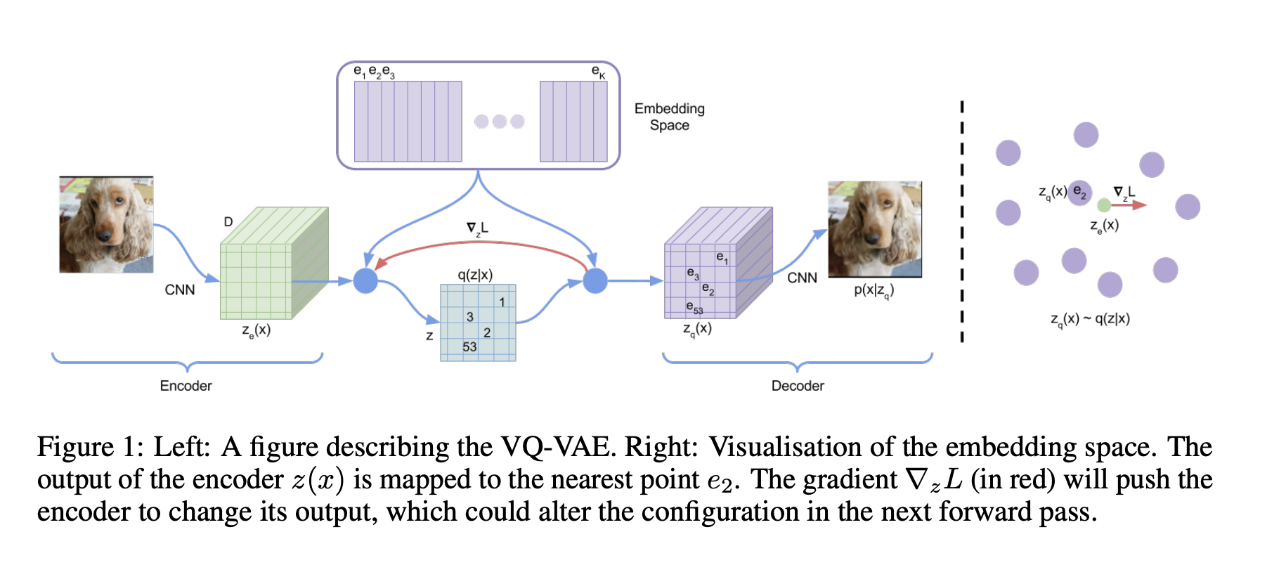
The posterior categorical distribution $q(z \mid x)$ probabilities are defined as one-hot as follows: $$ q(z=k \mid x)= \begin{cases}1 & \text { for } \mathrm{k}=\operatorname{argmin}_j\left\|z_e(x)-e_j\right\|_2, \\ 0 & \text { otherwise }\end{cases} $$ where $z_e(x)$ is the output of the encoder network. This model is viewed as a VAE in which we can bound $\log p(x)$ with the ELBO. Our proposal distribution $q(z=k \mid x)$ is deterministic, and by defining a simple uniform prior over $z$ we obtain a KL divergence constant and equal to $\log K$.

The representation $z_e(x)$ is passed through the discretisation bottleneck followed by mapping onto the nearest element of embedding $e$ as given in equations 1 and 2 . $$ z_q(x)=e_k, \quad \text { where } \quad k=\operatorname{argmin}_j\left\|z_e(x)-e_j\right\|_2 $$

We will be training encoder, decoder and embeddings simulaneously!

VQ-VAE: challenges and the loss

The distribution over categories is assumed in the original paper to be uniform.

This, KL-loss is constant an is not involved in optimization, so other losses are needed!

Instead, the following loss is used:

Thus, the total training objective becomes: $$ L=\log p\left(x \mid z_q(x)\right)+\left\|\operatorname{sg}\left[z_e(x)\right]-e\right\|_2^2+\beta\left\|z_e(x)-\operatorname{sg}[e]\right\|_2^2, $$

where $\operatorname{sg}$ is a stop-gradient operation (i.e. it is identity in the forward pass, and has zero partial derivatives in the backward pass).

The last loss, the commitment loss, which only applies to the encoder weights, encourages the output of the encoder to stay close to the chosen codebook vector to prevent it from fluctuating too frequently from one code vector to another

VQ-VAE: architecture

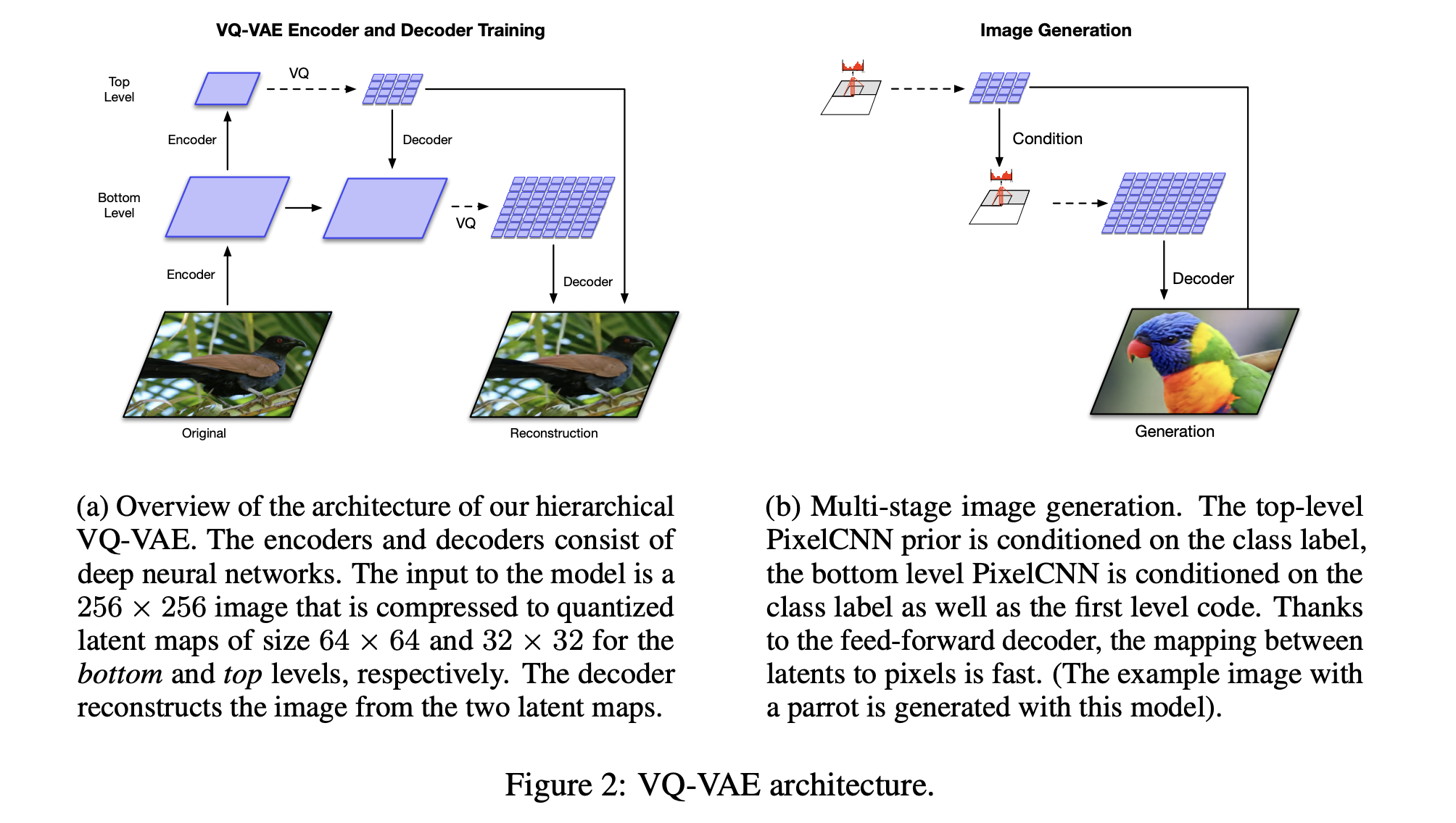
VQ-VAE version 2

The improvement of VQ-VAE scheme has been proposed in Generating Diverse High-Fidelity Images with VQ-VAE-2

It uses the same loss, but tries to learn hierarhical codes.

VQ-VAE version 2: stage 1

In the first stage, hierarchical latent codes are used.

For example, for 256 × 256 images, a two level latent hierarchy is used. The encoder network first transforms and downsamples the image by a factor of 4 to a 64 × 64 representation which is quantized to our bottom level latent map. Another stack of residual blocks then further scales down the representations by a factor of two, yielding a top-level 32 × 32 latent map after quantization.

The decoder is similarly a feed-forward network that takes as input all levels of the quantized latent hierarchy. It consists of a few residual blocks followed by a number of strided transposed convolutions to upsample the representations back to the original image size.

VQ-VAE version 2: stage 2

Once we have the encoder, we can model the distribution of the discrete latent

by a PixelCNN autoregressive architecture (in fact, PixelSnail approach with self-attention).

This is done independently.

Of course, one can use other discrete distribution models over those latents.

Scheme of the approache

Possible improvements over VQ-VAE

VQ-VAE architecture:

1. Uses uniform prior over discrete latent space
2. Separate learning of decoder/endocoder

One can easily use GPT to model the dependencies over the resulting latent variables, for example, as in VideoGPT paper, where GPT is used to predict the discrete latent codes.

VQ-GAN

Significant improvement of VQ-VAE has been achieved by combining the ideas of VQ-VAE with the ideas of generative networks (GANs), resulting in the VQ-GAN.

In short (we will cover this in the lecture on GANs) is to add an additional loss on the quality of the generated images, and the loss is borrowed from GANs.

Comparison with autoregressive models

• PixelCNN: tractable probability density functions
• VAE: intractable propability density functions, solved by variational inference.
• VQ-VAE: strictly speaking, encoder-decoder architecture with codebook lookup.

Summary

• Autoregressive models
• Variational Autoencoders

Next lecture: Generative models II

• Generative adversarial networks
• DCGAN
• WGAN
• StyleGAN
• Evaluating generative models