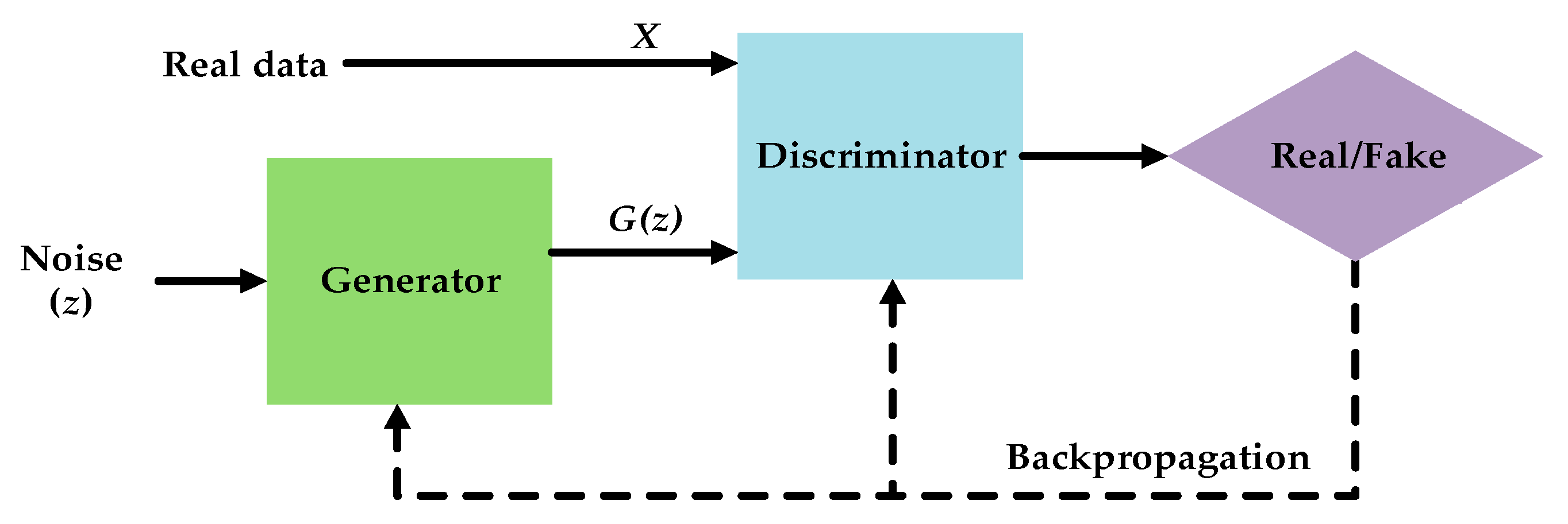
The original idea of Generative Adversarial Nets
has the following form: we treat the problem of distinguishing between real and fake samples as binary classification task.
We are considering the problem of learning a distribution from samples.
We parametrize the distribution as
$$G(z), z \sim p(z).$$So, we have access to real samples and fake samples (generated from the generator).
How we distinguish between them?
The original idea of Generative Adversarial Nets
has the following form: we treat the problem of distinguishing between real and fake samples as binary classification task.
We have a min-max problem: we want the discriminator to detect the fakes, whereas we want the generator to fool the discriminator
$$\min_G \max_D L(D, G), \quad L(D, G) = E_{x \sim p_{r}} \log D(x) + E_{z \sim p_z} \log(1-D(G(z))$$What the solution of this problem?
Suppose that real data has density $\rho_r$ and synthetic data has density $\rho_g$.
Then, we have
$$\int \rho_r(x) \log D(x) + \int \rho_g(x) \log (1 - D(x)).$$By optimizing over $D(x)$ we get
$$\frac{\rho_r}{D} - \frac{\rho_g}{1-D} = 0,$$$$\rho_g(1-D) - \rho_rD = 0, \quad D = \frac{\rho_r}{\rho_g + \rho_r}$$This is the optimal discriminator.
If we put the optimal discriminator into the formula, we get
$$L(G, D_*) = \int \rho_r \log \frac{\rho_r}{\rho_g + \rho_r} + \int \rho \log \frac{\rho_g}{\rho_g + \rho_r}$$For the optimal discriminator defined before, we have
$$L(G, D^*) = 2D_{JS}(p_{r} \| p_g) - 2\log2, $$where $D_{JS}$ is the Jensen-Shannon divergence (symmetrized version of the KL-divergence)
$$D_{JS}(p \| q) = \frac{1}{2} D_{KL}(p \| \frac{p + q}{2}) + \frac{1}{2} D_{KL}(q \| \frac{p + q}{2})$$Thus, minimization over $G$ will lead to $p_r = p_g$ if the generator is expressive enough,
and $D_* = \frac{1}{2}$.
In training a basic GAN, we:
Sometimes, in early training $G$ is quite poor and $\log(1 - D(G(z))$ saturates and it has been proposed to train $G$ to maximize $\log D(G(z))$ rather than minimize $\log(1 - D(G(z))$.
The gradients are much larger.
The problem with this 'non-saturating' loss is that it is heuristic and is not well-described by theory.
With the optimal $D_*$ in this case we have $$ \begin{array}{r} E_{x \sim p_g}\left[-\log \left(D_G^*(x)\right)\right]+E_{x \sim p_g}\left[\log \left(1-D_G^*(x)\right)\right] \\ =E_{x \sim p_g}\left[\log \frac{\left(1-D_G^*(x)\right)}{D_G^*(x)}\right]=E_{x \sim p_g}\left[\log \frac{p_g(x)}{p_{\text {data }}(x)}\right] \\ =K L\left(p_g \| p_{\text {data }}\right) . \end{array} $$
After putting it all together, we will get the following loss for $G$ as $$ \begin{aligned} & E_{x \sim p_g}\left[-\log \left(D_G^*(x)\right)\right] \\ & =K L\left(p_g \| p_{\text {data }}\right)-2 J S\left(p_{\text {data }} \| p_g\right) \\ & +E_{x \sim p_{\text {data }}}\left[\log D_G^*(x)\right]+2 \log 2 . \\ & \end{aligned} $$ The first loss minimizes the difference, while the second maximizes. This may result in unstable training for $G$.
Two extreme cases:
First error: $G$ produces implausible examples. The second error: generator produces insufficiently diverse ('safe' example). This problem is known as mode collapse.
Original GAN model involved MLP and is not scalable.
DeepConvolutional GAN was the first working GAN for large-scale image generation. It provided several recipes for building architectures and stable training,
such as
Wasserstein GAN was based on the idea of using another type of metric between distribution to minimize, namely the Wasserstein distance.
The Earth-Mover (EM) distance or Wasserstein-1 $$ W\left(\mathbb{P}_r, \mathbb{P}_g\right)=\inf _{\gamma \in \Pi\left(\mathbb{P}_r, \mathbb{P}_g\right)} \mathbb{E}_{(x, y) \sim \gamma}[\|x-y\|] $$ where $\Pi\left(\mathbb{P}_r, \mathbb{P}_g\right)$ denotes the set of all joint distributions $\gamma(x, y)$ whose marginals are respectively $\mathbb{P}_r$ and $\mathbb{P}_g$. Intuitively, $\gamma(x, y)$ indicates how much "mass" must be transported from $x$ to $y$ in order to transform the distributions $\mathbb{P}_r$ into the distribution $\mathbb{P}_g$. The EM distance then is the "cost" of the optimal transport plan.
Example 1 (Learning parallel lines). Let $Z \sim U[0,1]$ the uniform distribution on the unit interval. Let $\mathbb{P}_0$ be the distribution of $(0, Z) \in \mathbb{R}^2$ (a 0 on the x-axis and the random variable $Z$ on the y-axis), uniform on a straight vertical line passing through the origin. Now let $g_\theta(z)=(\theta, z)$ with $\theta$ a single real parameter. It is easy to see that in this case,
where $\delta$ is a Total Variation distance, defined as
$$ \delta\left(\mathbb{P}_r, \mathbb{P}_g\right)=\sup _{A \in \Sigma}\left|\mathbb{P}_r(A)-\mathbb{P}_g(A)\right| . $$As we see, the only 'smooth' is the Wasserstein distance.
Computing infimum in
$$ W\left(\mathbb{P}_r, \mathbb{P}_g\right)=\inf _{\gamma \in \Pi\left(\mathbb{P}_r, \mathbb{P}_g\right)} \mathbb{E}_{(x, y) \sim \gamma}[\|x-y\|] $$is intractable (or not easy at least). There is a Kantorovich duality representation of this distance as
$$ W\left(\mathbb{P}_r, \mathbb{P}_\theta\right)=\sup _{\|f\|_L \leq 1} \mathbb{E}_{x \sim \mathbb{P}_r}[f(x)]-\mathbb{E}_{x \sim \mathbb{P}_\theta}[f(x)] $$where the supremum is over all the 1-Lipschitz functions $f: \mathcal{X} \rightarrow \mathbb{R}$.
It is also sufficient to optimize over bounded-Lipschitz functions
The objective is similar to the GAN, but with the Lipschitz constraint.
The original WGAN paper proposed to use weight clipping to $[-c, c]$ (and confirmed it is a terrible idea).
A subsequent paper Improved Wasserstein GAN training uses gradient penalty instead
The resulting loss function has the form
$$L=\underbrace{\underset{\tilde{\boldsymbol{x}} \sim \mathbb{P}_g}{\mathbb{E}}[D(\tilde{\boldsymbol{x}})]-\underset{\boldsymbol{x} \sim \mathbb{P}_r}{\mathbb{E}}[D(\boldsymbol{x})]}_{\text {Original critic loss }}+\underbrace{\lambda \underset{\hat{\boldsymbol{x}} \sim \mathbb{P}_{\hat{\boldsymbol{x}}}}{\mathbb{E}}\left[\left(\left\|\nabla_{\hat{\boldsymbol{x}}} D(\hat{\boldsymbol{x}})\right\|_2-1\right)^2\right] .}_{\text {Our gradient penalty }}$$and $\hat{x}$ is sampled from straight lines between original samples and fake samples.
Another way of stabilizing GAN training is Spectral normalization
The idea is to introduce spectral norm bound on the weights (by doing power iteration)
Algorithm 1 SGD with spectral normalization
Spectral normalization is present in many GAN architectures nowdays, but it is not present in StyleGAN.
The cross-entropy is not a panacea. One can actually use different loss functions, for example Least Squares GAN
with the min-max problem of the form $$ \begin{aligned} \min _D V_{\mathrm{LSGAN}}(D) & =\frac{1}{2} \mathbb{E}_{\boldsymbol{x} \sim p_{\text {data }}(\boldsymbol{x})}\left[(D(\boldsymbol{x})-b)^2\right] \\ & +\frac{1}{2} \mathbb{E}_{\boldsymbol{z} \sim p_{\boldsymbol{z}}(\boldsymbol{z})}\left[(D(G(\boldsymbol{z}))-a)^2\right] \\ \min _G V_{\mathrm{LSGAN}}(G) & =\frac{1}{2} \mathbb{E}_{\boldsymbol{z} \sim p_{\boldsymbol{z}}(\boldsymbol{z})}\left[(D(G(\boldsymbol{z}))-c)^2\right] \end{aligned} $$
The resulting objective is smoother.
GANs are much more difficult to train, than standard networks due to the adversarial loss.
It can be shown, that min-max problems solved with gradient descent/ascent are prone to oscillatory behaviour
due to the presence of complex eigenvalues in the linearization of the model.
Many methods have been proposed to 'monotonize' the convergence, but most of them are not very functional.
If we train on a small dataset, the discriminator tends to overfit.
In Training Generative Adversarial Networks with Limited Data, by T. Karras et. al
it has been proposed to make problem more difficult for the discriminator by data augmentation.
Note, we need to use differentiable data augmentation.
The strength of augmentation also has to be determined.
It significantly improves on small and medium datasets!

The standard metrics for evaluating the qualities of generated images are:
Inception score has been proposed in Improved Techniques for Training GANs
The idea is to compute conditional label distribution $p(y \mid x)$ with an Inception model. Good images are assumed to have low-entropy, quantized by the formula
$$\exp \left(\mathbb{E}_{\boldsymbol{x}} \operatorname{KL}(p(y \mid \boldsymbol{x}) \| p(y))\right)$$By far the most popular metric, proposed in GANs Trained by a Two Time-Scale Update Rule Converge to a Local Nash Equilibrium
Disadvantage: it only compares two momemts of the distributions, thus ignoring higher-order topological representations.
In order to generate higher-resolution images, several approaches have been proposed.
In SAGAN (Self-attention GAN) a self-attention is built into the CNN architecture.
SAGAN was later scaled to BigGAN by using several engineering tricks.
The next step has been progressive growing of GANS, which we will discuss.
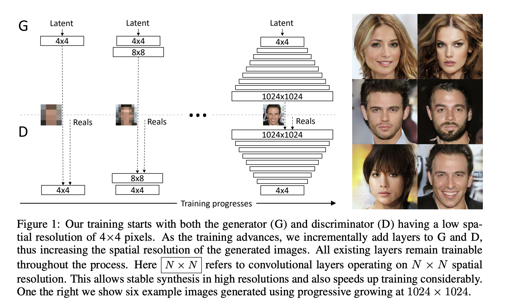
In Progressive Growing of GANs for Improved Quality, Stability, and Variation a new methodology for training GANs has been proposed.
The idea is to train on lower resolutions and add layers to $G$ and $D$.
Other techniques include minibatch discrimination
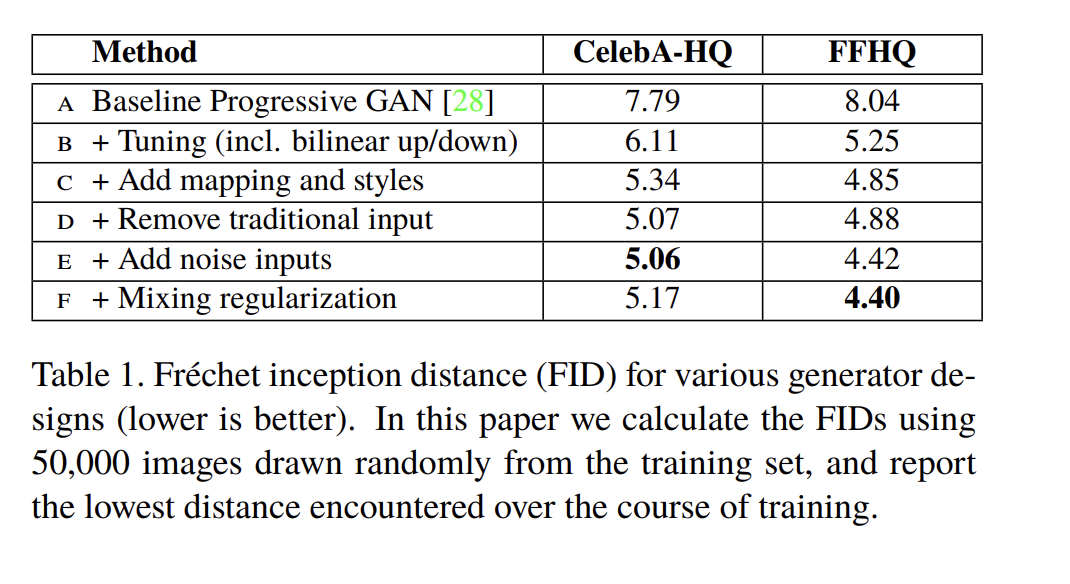
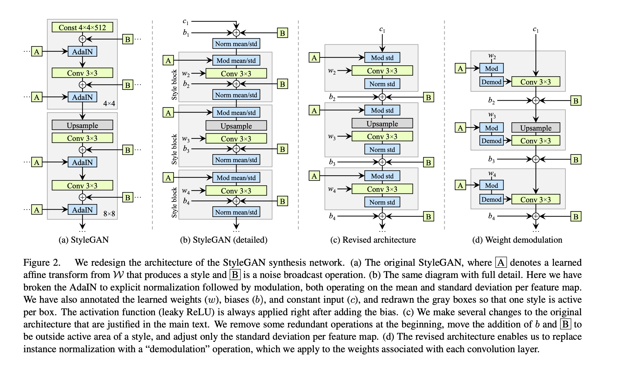
A Style-Based Generator Architecture for Generative Adversarial Networks by T. Karras et. al.
the StyleGAN architecture has been proposed.
The loss function and discriminator are the same, only generator (+few tricks) is redesigned to put noise in different resolutions.
One of the new block is Adaptive Normalization given as
$$\operatorname{AdaIN}\left(\mathbf{x}_i, \mathbf{y}\right)=\mathbf{y}_{s, i} \frac{\mathbf{x}_i-\mu\left(\mathbf{x}_i\right)}{\sigma\left(\mathbf{x}_i\right)}+\mathbf{y}_{b, i}$$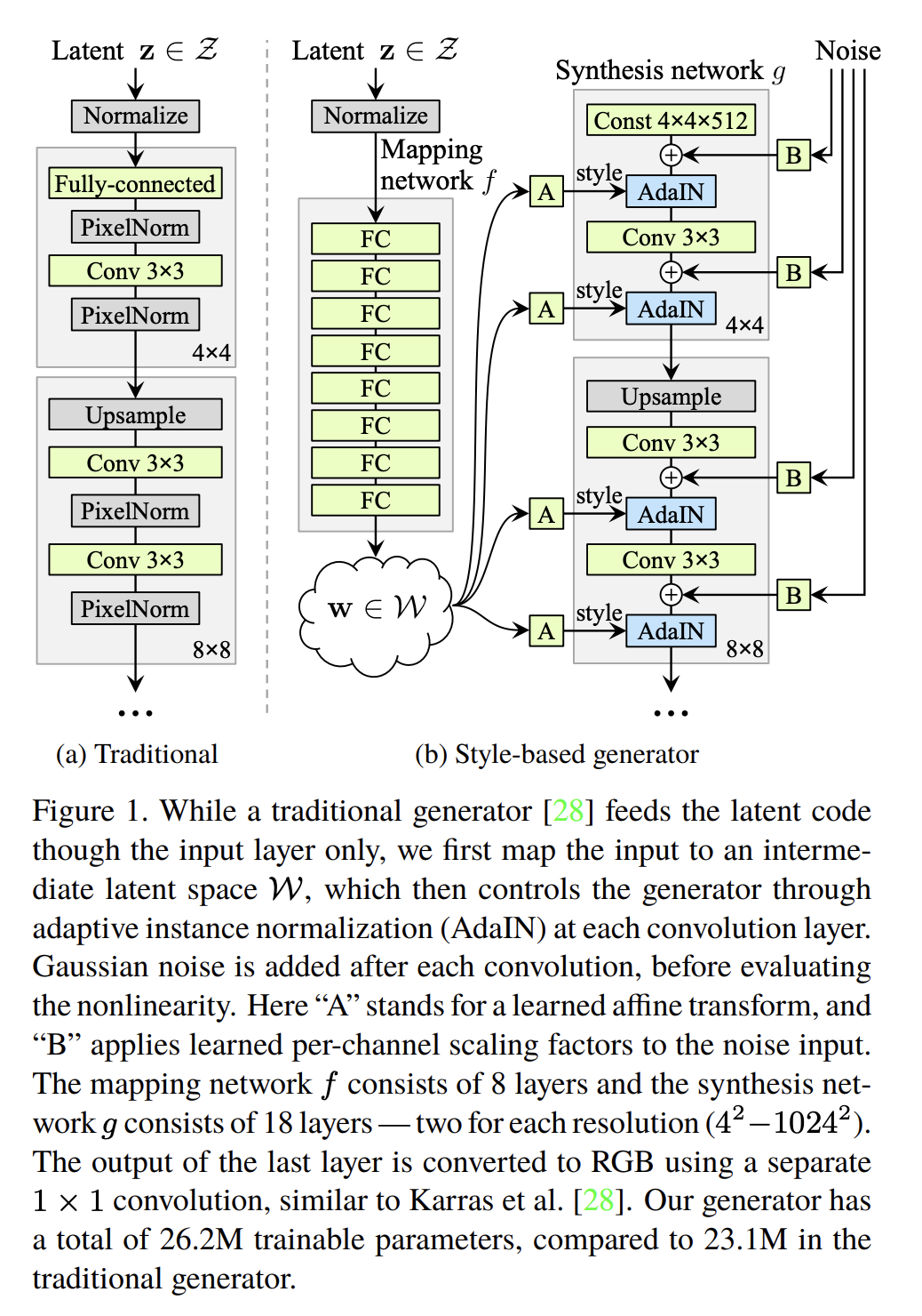
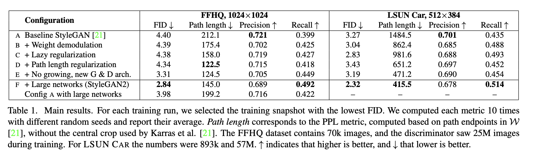
In Analyzing and Improving the Image Quality of StyleGAN the quality of generated images has improved even further.
At a single $\mathbf{w} \in \mathcal{W}$ the local metric scaling properties of the generator mapping $g(\mathbf{w}): \mathcal{W} \rightarrow \mathcal{Y}$ are captured by the Jacobian matrix $\mathbf{J}_{\mathbf{w}}=\delta g(\mathbf{w}) / \delta \mathbf{w}$. Motivated by the desire to preserve the expected lengths of vectors regardless of the direction, we formulate the regularizer as: $$ \mathbb{E}_{\mathbf{w}, \mathbf{y} \sim \mathcal{N}(0, \mathbf{I})}\left(\left\|\mathbf{J}_{\mathbf{w}}^{\mathbf{T}} \mathbf{y}\right\|_2-a\right)^2 $$ where $y$ are random images with normally distributed pixel intensities, and $w \sim f(z)$, where $z$ are normally distributed.
Conditional adversarial networks showed that it is quite easy to modify the generation subject to some conditioning information.
Instead of $p(x)$ we just model $p(x \mid y)$.
The original paper conditioned on the class, but you can also do image2image transformations!
Image-to-Image Translation with Conditional Adversarial Networks
shows how to modify GAN architecture for image-to-image translation.
A conditional GAN learns a mapping from a pair $\{x, z\}$ to the output $y$.
The objective of a conditional GAN can be expressed as $$ \begin{aligned} \mathcal{L}_{c G A N}(G, D)= & \mathbb{E}_{x, y}[\log D(x, y)]+ \\ & \mathbb{E}_{x, z}[\log (1-D(x, G(x, z))] \end{aligned} $$
Since we have to output something close to $y$, it is beneficial to add reconstruction loss to the model:
$$ \mathcal{L}_{L 1}(G)=\mathbb{E}_{x, y, z}\left[\|y-G(x, z)\|_1\right] $$Our final objective is $$ G^*=\arg \min _G \max _D \mathcal{L}_{c G A N}(G, D)+\lambda \mathcal{L}_{L 1}(G) $$
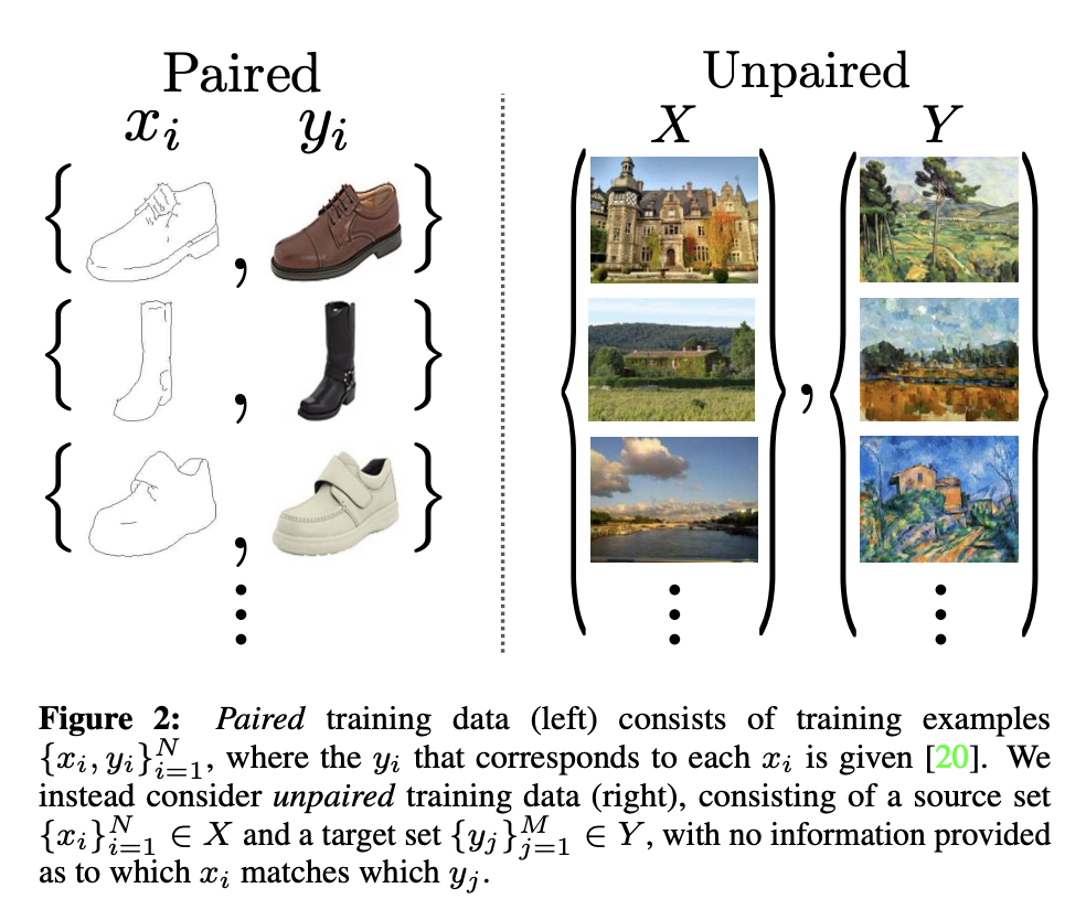
The approach described before requires a parallel corpus. GAN, however, learn distributions.
Can we learn a mapping without having paired data?
One of the seminal methods has been cycleGAN proposed in Unpaired image-to-image translation using cycle-consistent adversarial networks.
GAN-loss has the standard form: \begin{aligned} \mathcal{L}_{\mathrm{GAN}}\left(G, D_Y, X, Y\right) & =\mathbb{E}_{y \sim p_{\text {data }}(y)}\left[\log D_Y(y)\right] \\ & +\mathbb{E}_{x \sim p_{\text {data }}(x)}\left[\log \left(1-D_Y(G(x))\right]\right. \end{aligned}
Cycle consistency loss: \begin{aligned} \mathcal{L}_{\mathrm{cyc}}(G, F) & =\mathbb{E}_{x \sim p_{\text {data }}(x)}\left[\|F(G(x))-x\|_1\right] \\ & +\mathbb{E}_{y \sim p_{\text {data }}(y)}\left[\|G(F(y))-y\|_1\right] \end{aligned}
Full formulation:
\begin{aligned} \mathcal{L}\left(G, F, D_X, D_Y\right)= & \mathcal{L}_{\mathrm{GAN}}\left(G, D_Y, X, Y\right) \\ & +\mathcal{L}_{\mathrm{GAN}}\left(F, D_X, Y, X\right) \\ & +\lambda \mathcal{L}_{\mathrm{cyc}}(G, F) \end{aligned}
CycleGAN and cGAN with paired data can only learn for two domains.
The approach of StarGAN conditions the generation on the domain type with a single model.
The loss has 3 components: the adversarial loss, the reconstruction loss and the domain classification loss (obtain from the discriminator).
StarGAN also has 2 versions.
One of the problem of a GAN model is that it is not invertible easily.
There is a big review on the subject.
Given a real image $x$, it is not always possible to find $z$ such that $G(z) \approx x$.
For standard GAN, we can look for optimal $z$.
For StyleGAN, additionally, we can optimize over
A typical solution to this problem now for StyleGAN is to optimize over $W$ or even every style vector (named $W^{+}$).
The latent space of GANs has interesting structure.
One can find linear direction in it which corresponds to interpretable directions.
There are many papers on this and many way to disentangle such directions.
One of the has been proposed by Voynov and Babenko
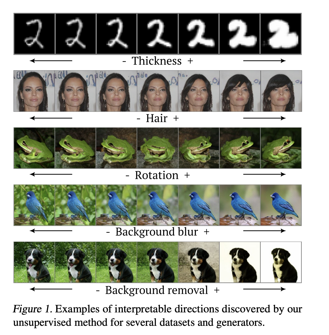
We need to find directions in the latent space that are interpretable.
We introduce an additional network $R$ (called reconstructor)
Reconstructor receives a pair $G(z), G(z + \varepsilon a_k)$ and tries to predict the shift.
$$\min _{A, R} \underset{z, k, \varepsilon}{\mathbb{E}} L(A, R)=\min _{A, R} \underset{z, k, \varepsilon}{\mathbb{E}}\left[L_{c l}(k, \widehat{k})+\lambda L_r(\varepsilon, \widehat{\varepsilon})\right]$$