Lecture 15: Generative models III (Score-based and diffusion models)

Previous lecture

• Generative adversarial networks
• DCGAN
• WGAN
• StyleGAN
• Evaluating generative models

Current lecture

• Score matching
• Denoising diffusion models
• Diffusion models and stochastic ordinary differential equations

Score matching

Score matching has been introduced in Song, Ermon, Generative Modeling by Estimating Gradients of the Data Distribution

Fisher divergence between two densities is defines as

$$E_p \Vert \nabla \log q - \nabla \log p \Vert^2$$

In score matching, we learn the score function $s_{\theta} = \nabla \log q$.

The objective minimizes $\frac{1}{2} \mathbb{E}_{p_{\text {data }}}\left[\left\|\mathbf{s}_{\boldsymbol{\theta}}(\mathbf{x})-\nabla_{\mathbf{x}} \log p_{\text {data }}(\mathbf{x})\right\|_2^2\right]$, which can be shown equivalent to the following up to a constant $$ \mathbb{E}_{p_{\text {data }}(\mathbf{x})}\left[\operatorname{tr}\left(\nabla_{\mathbf{x}} \mathbf{s}_{\boldsymbol{\theta}}(\mathbf{x})\right)+\frac{1}{2}\left\|\mathbf{s}_{\boldsymbol{\theta}}(\mathbf{x})\right\|_2^2\right] $$

The main challenge is in the evaluation of the trace of the Jacobian.

Approximating the trace: denoising score matching

There are two ways of approximation of the trace. The first is called denoising score matching and is based on the well-known approximation of the Jacobian.

The objective is written as

\begin{equation} \frac{1}{2} \mathbb{E}_{q_\sigma(\tilde{\mathbf{x}} \mid \mathbf{x}) p_{\text {data }}(\mathbf{x})}\left[\left\|\mathbf{s}_{\boldsymbol{\theta}}(\tilde{\mathbf{x}})-\nabla_{\tilde{\mathbf{x}}} \log q_\sigma(\tilde{\mathbf{x}} \mid \mathbf{x})\right\|_2^2\right] \end{equation}

where \begin{equation} q_\sigma(\tilde{\mathbf{x}} \mid \mathbf{x}) \end{equation} is the predefined noise distribution and

\begin{equation} q_\sigma(\tilde{\mathbf{x}}) \triangleq \int q_\sigma(\tilde{\mathbf{x}} \mid \mathbf{x}) p_{\mathrm{data}}(\mathbf{x}) \mathrm{d} \mathbf{x} \end{equation}

Approximating the trace: sliced score matching

We can also approximate the trace by using Hutchinson trace estimator.

The objective reads

\begin{equation} \mathbb{E}_{p_{\mathbf{v}}} \mathbb{E}_{p_{\text {data }}}\left[\mathbf{v}^{\top} \nabla_{\mathbf{x}} \mathbf{s}_{\boldsymbol{\theta}}(\mathbf{x}) \mathbf{v}+\frac{1}{2}\left\|\mathbf{s}_{\boldsymbol{\theta}}(\mathbf{x})\right\|_2^2\right] \end{equation}

The term inside can be efficiently computed using autodifferentiation, and $p_v$ is a simple distribution (i.e., normal distribution).

Sampling

Suppose we know $s_{\theta}(x) \approx \nabla \log p$.

Then, how we sample from such kind of distribution?

One of the classical approaches is Langevin sampling.

If we know the gradient of the logarithm of $p$, the following procedure will lead to samples of $p$:

The Langevin method recursively computes the following $$ \tilde{\mathbf{x}}_t=\tilde{\mathbf{x}}_{t-1}+\frac{\epsilon}{2} \nabla_{\mathbf{x}} \log p\left(\tilde{\mathbf{x}}_{t-1}\right)+\sqrt{\epsilon} \mathbf{z}_t, $$ where $\mathbf{z}_t \sim \mathcal{N}(0, I)$. The distribution of $\tilde{\mathbf{x}}_T$ equals $p(\mathbf{x})$ when $\epsilon \rightarrow 0$ and $T \rightarrow \infty$, in which case $\tilde{\mathbf{x}}_T$ becomes an exact sample from $p(\mathbf{x})$ under some regularity conditions. When $\epsilon>0$ and $T<\infty$, a Metropolis-Hastings update is needed to correct the error in the equation above, but it can often be ignored in practice.

Original idea of diffusion models

The original idea of diffusion model has been proposed in 2015 in the paper Jascha Sohl-Dickstein, Eric Weiss, Niru Maheswaranathan, and Surya Ganguli. Deep unsupervised learning using nonequilibrium thermodynamic.

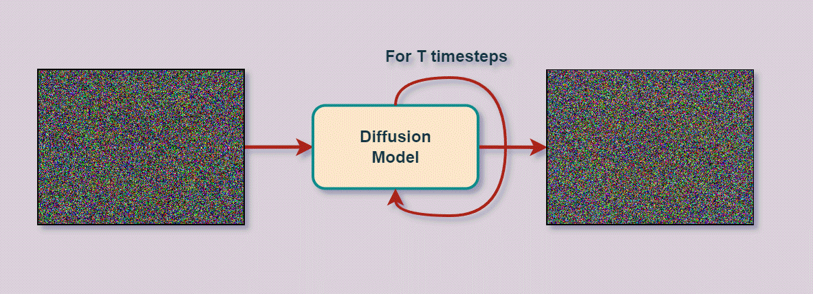
We sequentially 'noise' the distribution in order to get to the right one.

This can be defined by a whole family of distrubutions.

The final result may look like this

Mathematical formalism

We need to define:

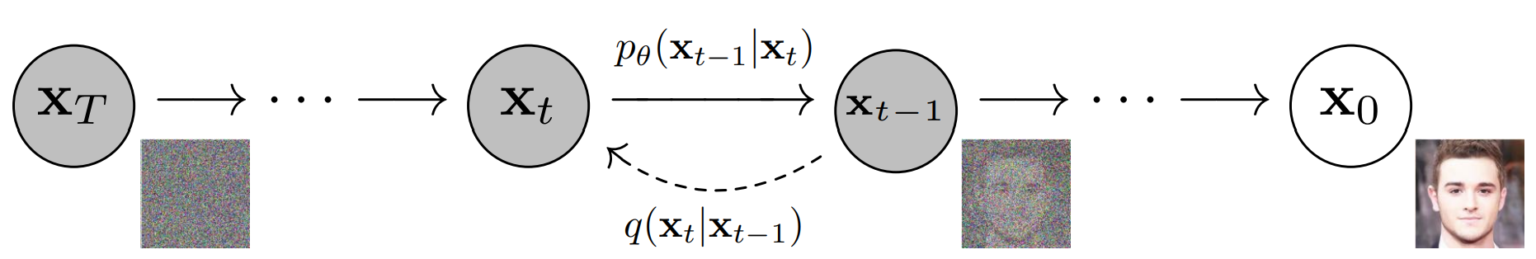
• $q(x_t \mid x_{t-1})$ Known as forward diffusion kernel, defines the probability density function (PDF) of the image at timestep $t$ conditioned on $x_{t-1}$. Note that it typically does not have any learnable parameters.
• $p_{\theta}(x_{t-1} \mid x_t)$ -- reverse diffusion kernel, the parameters $\theta$ are learned using neural network architecture.

How the forward diffusion is defined

Modern deep denoising diffusion has been introduced in Denoising Diffusion Probabilistic Models by Jonathan Ho, Ajay Jain, Pieter Abbeel, Neurips2020 and called Denosing Diffusion Probabilistic Models (DDPM).

The forward process is parametrized as a Markov chain:

\begin{equation} \begin{aligned} q\left(x_1, \ldots, x_T \mid x_0\right) & :=\prod_{t=1}^T q\left(x_t \mid x_{t-1}\right) \\ q\left(x_t \mid x_{t-1}\right) & :=\mathcal{N}\left(x_t ; \sqrt{1-\beta_t} x_{t-1}, \beta_t I\right) \end{aligned} \end{equation}

The meaning of the forward process is extremely simple.

Can you describe it?

The samples from the PDF at time $t$ can be computed as

$$ x_t=\sqrt{1-\beta_t} x_{t-1}+\sqrt{\beta_t} \epsilon, $$

where $\epsilon \sim \mathcal{N}(0, I)$

Parameter $\beta_t$ is called diffusion rate.

Note, that in order to sample $x_t$, we need to sample $x_0, \ldots, x_{t-1}$ which can be time-consuming.

Instead, we can sample from $q(x_t \mid x_0)$ directly, since it is also a Gaussian:

\begin{equation} \begin{aligned} q\left(x_t \mid x_0\right) & :=\mathcal{N}\left(x_t ; \sqrt{\bar{\alpha}_t} x_{t-1},\left(1-\bar{\alpha}_t\right) I\right) \\ x_t & :=\sqrt{\bar{\alpha}_t} x_0+\sqrt{1-\bar{\alpha}_t} \epsilon \end{aligned} \end{equation}

where

\begin{equation} \begin{aligned} \alpha_t & :=1-\beta_t \\ \bar{\alpha}_t & :=\prod_{s=1}^t \alpha_s \end{aligned} \end{equation}

In the end, $q(x_T) = N(x_t, 0, I)$.

Reverse diffusion process

The reverse process is the integral over all possible pathways to arrive a data sample.

\begin{equation} \begin{gathered} p_\theta\left(x_0\right):=\int p_\theta\left(x_{0: T}\right) d x_{1: T} \\ p_\theta\left(\mathbf{x}_{0: T}\right):=p\left(\mathbf{x}_T\right) \prod_{t=1}^T p_\theta\left(\mathbf{x}_{t-1} \mid \mathbf{x}_t\right), \quad p_\theta\left(\mathbf{x}_{t-1} \mid \mathbf{x}_t\right):=\mathcal{N}\left(\mathbf{x}_{t-1} ; \boldsymbol{\mu}_\theta\left(\mathbf{x}_t, t\right), \mathbf{\Sigma}_\theta\left(\mathbf{x}_t, t\right)\right) \end{gathered} \end{equation}

Training objective

We can try to maximize the likelihood!

\begin{equation} \begin{aligned} p_\theta\left(x_0\right) & :=\int p_\theta\left(x_{0: T}\right) d x_{1: T} \\ L & =-\log \left(p_\theta\left(x_0\right)\right) \end{aligned} \end{equation}

This likelihood is intractable. So what can we do?

Use ELBO!

ELBO for DDPM

\begin{equation} \mathbb{E}\left[-\log p_\theta\left(\mathbf{x}_0\right)\right] \leq \mathbb{E}_q\left[-\log \frac{p_\theta\left(\mathbf{x}_{0: T}\right)}{q\left(\mathbf{x}_{1: T} \mid \mathbf{x}_0\right)}\right]=\mathbb{E}_q\left[-\log p\left(\mathbf{x}_T\right)-\sum_{t \geq 1} \log \frac{p_\theta\left(\mathbf{x}_{t-1} \mid \mathbf{x}_t\right)}{q\left(\mathbf{x}_t \mid \mathbf{x}_{t-1}\right)}\right]=: L \end{equation}

It can be rewritten as

\begin{equation} \mathbb{E}_q[\underbrace{D_{\mathrm{KL}}\left(q\left(\mathbf{x}_T \mid \mathbf{x}_0\right) \| p\left(\mathbf{x}_T\right)\right)}_{L_T}+\sum_{t>1} \underbrace{D_{\mathrm{KL}}\left(q\left(\mathbf{x}_{t-1} \mid \mathbf{x}_t, \mathbf{x}_0\right) \| p_\theta\left(\mathbf{x}_{t-1} \mid \mathbf{x}_t\right)\right)}_{L_{t-1}} \underbrace{-\log p_\theta\left(\mathbf{x}_0 \mid \mathbf{x}_1\right)}_{L_0}] \end{equation}

and represented as a sum:

\begin{equation} \begin{aligned} L_{\mathrm{vlb}} & :=L_0+L_1+\ldots+L_{T-1}+L_T \\ L_0 & :=-\log p_\theta\left(x_0 \mid x_1\right) \\ L_{t-1} & :=D_{K L}\left(q\left(x_{t-1} \mid x_t, x_0\right) \| p_\theta\left(x_{t-1} \mid x_t\right)\right) \\ L_T & :=D_{K L}\left(q\left(x_T \mid x_0\right) \| p\left(x_T\right)\right) \end{aligned} \end{equation}

The authors then ignore $L_0$ and it is obvious we can ignore $L_T$.

Thus, only $L_{t-1}$ is left.

\begin{equation} L_{v l b}:=L_{t-1}:=D_{K L}\left(q\left(x_{t-1} \mid x_t, x_0\right)|| p_\theta\left(x_{t-1} \mid x_t\right)\right) \end{equation}

This objective is quite natural.

Simplifying the bound

The function $q(x_{t-1} \mid x_t, x_0)$ can be written as

$$ q\left(\mathbf{x}_{t-1} \mid \mathbf{x}_t, \mathbf{x}_0\right)=\mathcal{N}\left(\mathbf{x}_{t-1} ; \tilde{\boldsymbol{\mu}}_t\left(\mathbf{x}_t, \mathbf{x}_0\right), \tilde{\beta}_t \mathbf{I}\right) $$

where $\quad \tilde{\boldsymbol{\mu}}_t\left(\mathbf{x}_t, \mathbf{x}_0\right):=\frac{\sqrt{\bar{\alpha}_{t-1}} \beta_t}{1-\bar{\alpha}_t} \mathbf{x}_0+\frac{\sqrt{\alpha_t}\left(1-\bar{\alpha}_{t-1}\right)}{1-\bar{\alpha}_t} \mathbf{x}_t \quad$ and $\quad \tilde{\beta}_t:=\frac{1-\bar{\alpha}_{t-1}}{1-\bar{\alpha}_t} \beta_t$

The authors of DDPM then set $\Sigma$ to be $\sigma^2 I$, simplifying everything to:

\begin{equation} \begin{gathered} p_\theta\left(x_{t-1} \mid x_t\right)=\mathcal{N}\left(x_{t-1} ; \mu_\theta\left(x_t, t\right), \Sigma_\theta\left(x_t, t\right)\right) \\ \downarrow \\ p_\theta\left(x_{t-1} \mid x_t\right)=\mathcal{N}\left(x_{t-1} ; \mu_\theta\left(x_t, t\right), \sigma^2 I\right) \end{gathered} \end{equation}

Since the variance is constant, the KL divergence is just the distance between the mean values, leaving the following objective:

\begin{equation} L_{t-1}=\mathbb{E}_q\left[\frac{1}{2 \sigma_t^2}\left\|\tilde{\boldsymbol{\mu}}_t\left(\mathbf{x}_t, \mathbf{x}_0\right)-\boldsymbol{\mu}_\theta\left(\mathbf{x}_t, t\right)\right\|^2\right]+C \end{equation}

The next step is to rewrite everything in terms of the noise:

$$ \bar{\mu}\left(x_t, x_0\right)=\frac{1}{\sqrt{\overline{x_t}}}\left(x_t-\frac{\beta_t}{\sqrt{1-\overline{\alpha_t}}} \epsilon_t\right) $$

Similarly, the formulation for $\mu_\theta\left(x_t, t\right)$ is set to: $$ \mu_\theta\left(x_t, x_0\right)=\frac{1}{\sqrt{\overline{x_t}}}\left(x_t-\frac{\beta_t}{\sqrt{1-\overline{\alpha_t}}} \epsilon_\theta\left(x_t, t\right)\right) $$

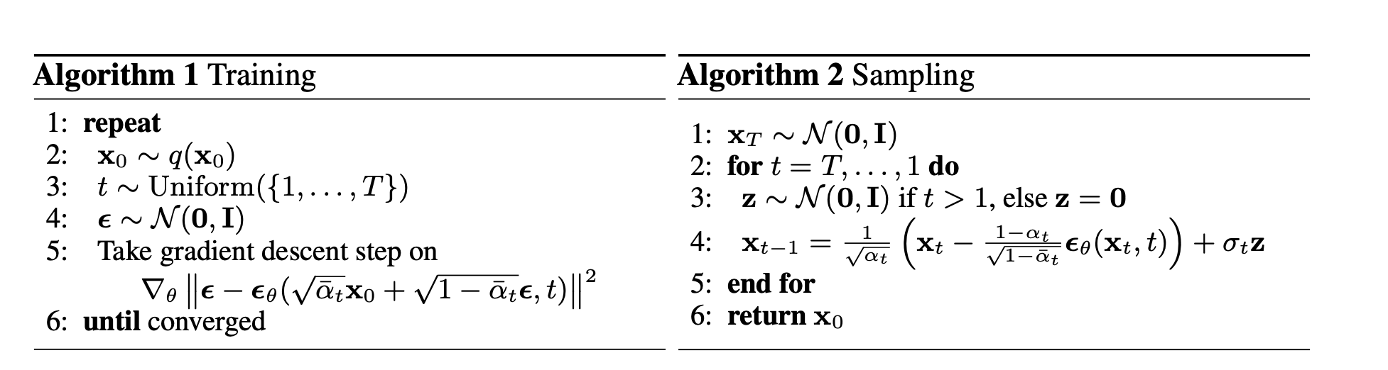
After another simplifying assumptions, they arrived at the loss function

\begin{equation} L_{\text {simple }}(\theta):=\mathbb{E}_{t, \mathbf{x}_0, \boldsymbol{\epsilon}}\left[\left\|\boldsymbol{\epsilon}-\boldsymbol{\epsilon}_\theta\left(\sqrt{\bar{\alpha}_t} \mathbf{x}_0+\sqrt{1-\bar{\alpha}_t} \boldsymbol{\epsilon}, t\right)\right\|^2\right] \end{equation}

I.e. we just try to fit the noise given the noised image.

Final algorithm

The algorithm for training and sampling is short and concise.

Architecture for the DDPM

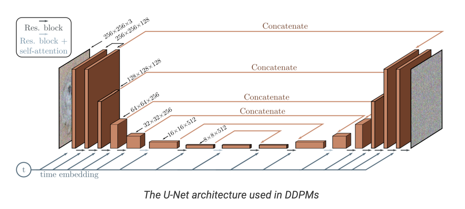
We have to parametrize image-to-image network $\varepsilon_{\theta}$ conditioned on the timestep $t$.

A good choice is UNet model.

The authors used UNet with Residual blocks with self-attention.

Details

• There are four levels in the encoder and decoder path with bottleneck blocks between them.
• Each encoder stage comprises two residual blocks with convolutional downsampling except the last level.
• Each corresponding decoder stage comprises three residual blocks and uses 2x nearest neighbors with convolutions to upsample the input from the previous level.
• Each stage in the encoder path is connected to the decoder path with the help of skip connections.
• The model uses “Self-Attention” modules at a single feature map resolution.
• Every residual block in the model gets the inputs from the previous layer (and others in the decoder path) and the embedding of the current timestep. The timestep embedding informs the model of the input’s current position in the Markov chain.

Improved DDPM models

Improved Denoising Diffusion Probabilistic Models improves over the original DDPMs. The FID score of the DDPM was great, but log-likelihood was not the best. The latter is responsible for mode collapse.

It tries to empricically parametrize the variance as \begin{equation} \Sigma_\theta\left(x_t, t\right)=\exp \left(v \log \beta_t+(1-v) \log \tilde{\beta}_t\right) \end{equation}

and modify the loss function as

\begin{equation} L_{\mathrm{hybrid}}=L_{\text {simple }}+\lambda L_{\text {vlb }} \end{equation}

A different noise schedule: \begin{equation} \bar{\alpha}_t=\frac{f(t)}{f(0)}, \quad f(t)=\cos \left(\frac{t / T+s}{1+s} \cdot \frac{\pi}{2}\right)^2 \end{equation}

Score-based diffusion modelling

DDPM is a discrete process. It can be viewed as a discretization of the stochastic differential equation (SDE), as described in

Score-Based Generative Modeling through Stochastic Differential Equations

We will provide a simpler and more concise derivation.

SDE

Lets start from the continous noising process:

\begin{equation} \mathrm{d} \mathbf{x}=\mathbf{f}(\mathbf{x}, t) \mathrm{d} t+\mathbf{G}(\mathbf{x}, t) \mathrm{d} \mathbf{w} \end{equation}

where $\mathrm{d} \mathbf{w}$ is a Wiener process.

We can use $f(x) = -x$, $g(x) = 1$ for example.

If we sample $x_0$ from a certain distribution $\rho_0 = \rho(0, x)$, it will induce the distribution $\rho(x, t)$ at time $t$.

This density will satisfy the Fokker-Planck equation:

where $\mathbf{f}(\cdot, t): \mathbb{R}^d \rightarrow \mathbb{R}^d$ and $\mathbf{G}(\cdot, t): \mathbb{R}^d \rightarrow \mathbb{R}^{d \times d}$. The marginal probability density $p_t(\mathbf{x}(t))$ evolves according to Kolmogorov's forward equation (Fokker-Planck equation) $$ \frac{\partial p_t(\mathbf{x})}{\partial t}=-\sum_{i=1}^d \frac{\partial}{\partial x_i}\left[f_i(\mathbf{x}, t) p_t(\mathbf{x})\right]+\frac{1}{2} \sum_{i=1}^d \sum_{j=1}^d \frac{\partial^2}{\partial x_i \partial x_j}\left[\sum_{k=1}^d G_{i k}(\mathbf{x}, t) G_{j k}(\mathbf{x}, t) p_t(\mathbf{x})\right] $$

Fokker-Planck equation

$$ \frac{\partial p_t(\mathbf{x})}{\partial t}=-\sum_{i=1}^d \frac{\partial}{\partial x_i}\left[f_i(\mathbf{x}, t) p_t(\mathbf{x})\right]+\frac{1}{2} \sum_{i=1}^d \sum_{j=1}^d \frac{\partial^2}{\partial x_i \partial x_j}\left[\sum_{k=1}^d G_{i k}(\mathbf{x}, t) G_{j k}(\mathbf{x}, t) p_t(\mathbf{x})\right] $$

The first term correspond to deterministic drift, the second -- to stochastic diffusion. The stochastic diffusion can not be reversed in a simple way.

Assume now that $\mathbf{G}$ = I.

Then we have the equation

$$ \frac{\partial p_t(\mathbf{x})}{\partial t} = - \nabla (f p_t) + \nabla^2 p_t. $$

We can rewrite it as

$$ \frac{\partial p_t(\mathbf{x})}{\partial t} = - \nabla (f p_t + p_t \nabla \log p_t), $$

i.e. which correponds to the deterministic drift

\begin{equation} \mathrm{d} \mathbf{x}=\mathbf{\hat{f}}(\mathbf{x}, t) \mathrm{d} t, \end{equation}

where

\begin{equation} \mathbf{\hat{f}}(\mathbf{x}, t) = \mathbf{f}(\mathbf{x}, t) - \nabla \log p_t(x, t). \end{equation}

What does it mean

We have a deterministic ODE that gives the same marginal densities as the stochastic ODE!

\begin{equation} \mathrm{d} \mathbf{x}=\mathbf{\hat{f}}(\mathbf{x}, t) \mathrm{d} t, \end{equation}

where

\begin{equation} \mathbf{\hat{f}}(\mathbf{x}, t) = \mathbf{f}(\mathbf{x}, t) - \nabla \log p_t(x, t). \end{equation}

But this ODE can be reversed.

The only thing we need to learn is the gradient $\nabla \log p_t(x, t)$.

We can learn it using score matching, since we know how to sample from $p_t$ if $\mathbf{f}(x) = -x$ (everything will be normal).

General form of the reverse SDE and computing the likelihood.

The general form of the inverse SDE is given as $$ \mathrm{d} \mathbf{x}=\underbrace{\left\{\mathbf{f}(\mathbf{x}, t)-\frac{1}{2} \nabla \cdot\left[\mathbf{G}(\mathbf{x}, t) \mathbf{G}(\mathbf{x}, t)^{\top}\right]-\frac{1}{2} \mathbf{G}(\mathbf{x}, t) \mathbf{G}(\mathbf{x}, t)^{\top} \mathbf{s}_{\boldsymbol{\theta}}(\mathbf{x}, t)\right\}}_{=: \tilde{f}_\theta(\mathbf{x}, t)} \mathrm{d} t . $$ With the instantaneous change of variables formula, we can compute the loglikelihood of $p_0(\mathbf{x})$ using $$ \log p_0(\mathbf{x}(0))=\log p_T(\mathbf{x}(T))+\int_0^T \nabla \cdot \tilde{\mathbf{f}}_{\boldsymbol{\theta}}(\mathbf{x}(t), t) \mathrm{d} t $$

It still requires the solution of ODEs.

Making diffusion models SOTA

By using architecture search, this paper achieved SOTA for image synthesis with diffusion models.

It

• Uses Adaptive Group Normalization to add information about time in correct place
• Proposed classifier guidance which includes the class information into the normalization as well.

The guidance makes the density dependent on the class label $y$, and also be made for the text-to-image generation as well!

Classifier guidance

Prior to classifier guidance, it was not known how to generate “low temperature” samples from a diffusion model.

Low-temperature means for GAN that reducing the variance of the latent variable, we get more high-quality samples (but less diverse). Instead, we can try to generate sample that are 'closer' to some predefined classes. The class is defined by a another pretrained classifier model.

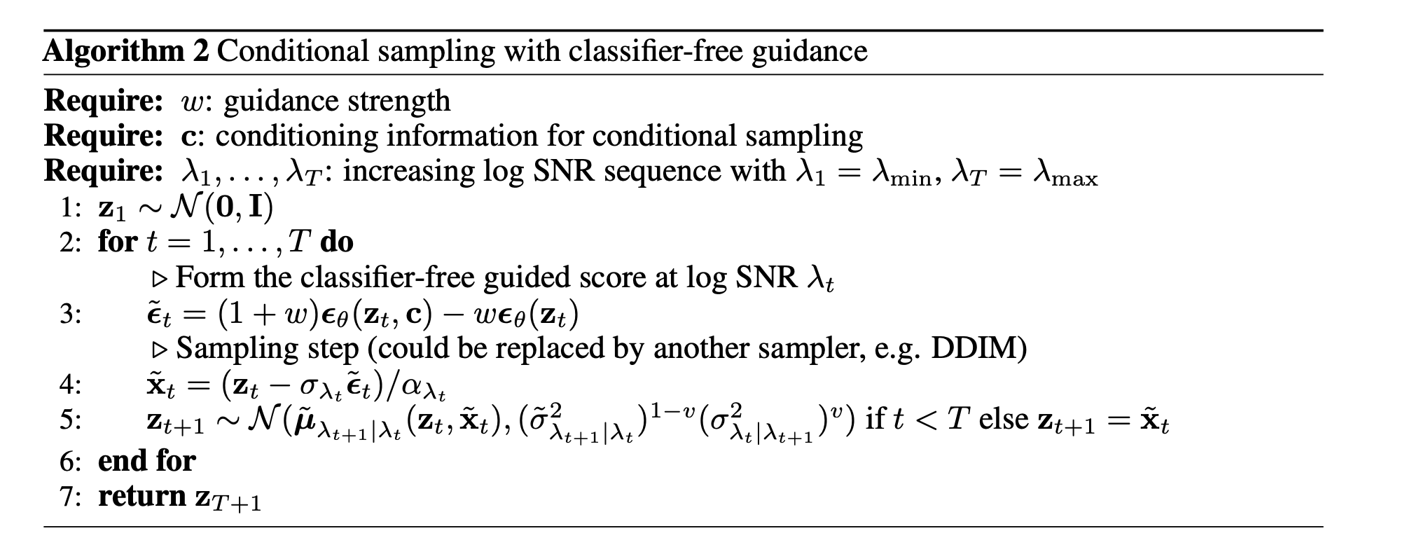
Classifier guidance:

The score given as \begin{equation}\boldsymbol{\epsilon}_\theta\left(\mathbf{z}_\lambda, \mathbf{c}\right) \approx-\sigma_\lambda \nabla_{\mathbf{z}_\lambda} \log p\left(\mathbf{z}_\lambda \mid \mathbf{c}\right) \end{equation} is modified to include the gradient of the $\log$ likelihood of an auxiliary classifier model $p_\theta\left(\mathbf{c} \mid \mathbf{z}_\lambda\right)$ as follows: $$ \tilde{\boldsymbol{\epsilon}}_\theta\left(\mathbf{z}_\lambda, \mathbf{c}\right)=\boldsymbol{\epsilon}_\theta\left(\mathbf{z}_\lambda, \mathbf{c}\right)-w \sigma_\lambda \nabla_{\mathbf{z}_\lambda} \log p_\theta\left(\mathbf{c} \mid \mathbf{z}_\lambda\right) \approx-\sigma_\lambda \nabla_{\mathbf{z}_\lambda}\left[\log p\left(\mathbf{z}_\lambda \mid \mathbf{c}\right)+w \log p_\theta\left(\mathbf{c} \mid \mathbf{z}_\lambda\right)\right], $$ where $w$ is a parameter that controls the strength of the classifier guidance. This modified score $\tilde{\boldsymbol{\epsilon}}_\theta\left(\mathbf{z}_\lambda, \mathbf{c}\right)$ is then used in place of $\boldsymbol{\epsilon}_\theta\left(\mathbf{z}_\lambda, \mathbf{c}\right)$ when sampling from the diffusion model, resulting in approximate samples from the distribution $$ \tilde{p}_\theta\left(\mathbf{z}_\lambda \mid \mathbf{c}\right) \propto p_\theta\left(\mathbf{z}_\lambda \mid \mathbf{c}\right) p_\theta\left(\mathbf{c} \mid \mathbf{z}_\lambda\right)^w . $$

Classifier-free guidance

In paper a classifier-free guidance is proposed.

It simulaneously trains a conditional and unconditional diffusion model (using a single network for that).

Sampling is performed by taking a linear combination of conditional and unconditional score estimates!

Challenges with diffusion models

• They are very compute-intensive: the initial implementation used 1000 steps, i.e. 1000 applications of UNet.
• Later research reduced it to 4-10 evaluations of the score function model, based on different ideas from numerical ODE solvers.
• Took 150-1000 V100 GPU-days.

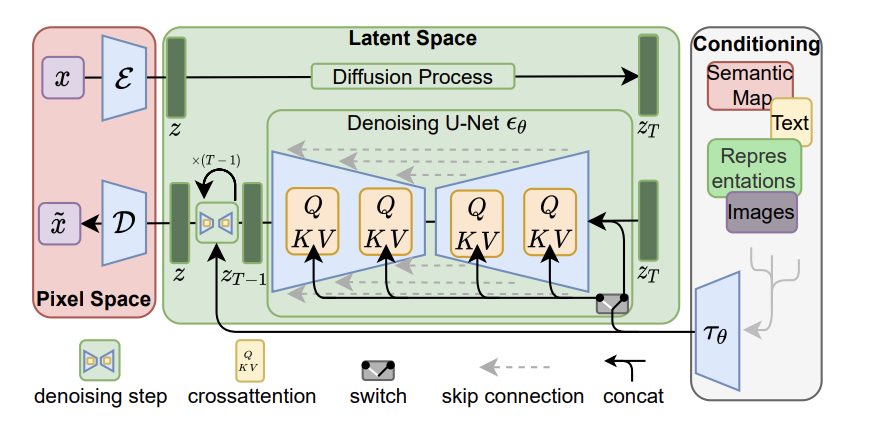
Latent diffusion models and democratizing the diffusion

The diffusion process occurring in the pixel space is time-consuming.

Pioneering paper showed that you can project the input image to the latent space, learn the diffusion model in the latent space and go back!

The encoder effectively downsamples the image, leaving the 2D structure.

The conditioning is enforced by cross-attention of the UNet-backbone with the conditioning features!

Diffusion models for other domains

The diffusion model has been extended to other domains with continuous input data.

It also has been extended to the discrete domain.

The noising process is replaced by mapping to uniform distribution or absorbing state.

Still in infancy.

Existing large diffusion models

• Dall-E 2: Dall-E 2 revealed in April 2022, generated even more realistic images at higher resolutions than the original Dall-E.
• Imagen is Google’s May 2022, version of a text-to-image diffusion model, which is not available to the public.
• Stable Diffusion: In August 2022, Stability AI released Stable Diffusion, an open-source Diffusion model similar to Dall-E 2 and Imagen. Stability AI’s released open source code and model weights, opening up the models to the entire AI community. Stable Diffusion was trained on an open dataset, using the 2 billion English label subset of the CLIP-filtered image-text pairs open dataset LAION 5b, a general crawl of the internet created by the German charity LAION.
• Midjourney is another diffusion model released in July 2022 and available via API and a discord bot.
• Kandinsky: Diffusion model of Sber.

Summary

• Score-based models
• Denoising diffusion models
• Diffusion models and stochastic differential equations