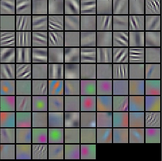
Convolutional neural networks in more details:
The first layer of the AlexNet model gives the following filters.
They are nice and smooth, which indicates the network has trained!
Note, that there are other visualization tools for the inner parameters of artificial neural networks!
The convolutions have problems with the boundary; If we do it many times, it will reduce the width and height of the image.
A typical solution is too add pixels around the border.
We can also shift the window not by 1 row/column, but by larger strides. This will downsample the object.
The first convolutional neural network architecture architecture was LeNet (tested on MNIST dataset).
What is average pooling ?
#Demo of adaptive & average poolingx
m = nn.AdaptiveAvgPool2d((5, 7))
input = torch.randn(1, 64, 8, 9)
output = m(input)
print(output.shape)
# target output size of 7x7 (square)
m = nn.AdaptiveAvgPool2d(7)
input = torch.randn(1, 64, 10, 9)
output = m(input)
# target output size of 10x7
m = nn.AdaptiveAvgPool2d((None, 7))
input = torch.randn(1, 64, 10, 9)
output = m(input)
torch.Size([1, 64, 5, 7])
LeNet has been tested on MNIST dataset (handwritten digits, 60000 samples).
This is an easy task.
Later, more complicated datasets have been introduced (CIFAR-10, CIFAR-100, Pascal VOC).
But they were still small and low-resolution, deep learning at that moment did not seem very promising for them.
In 2006, Fei-Fei Li proposed the creation of an ImageNet dataset.
'While most of the people pay attention to models, lets pay attention to data'.
In July 2008, ImageNet had zero images. By December, it had categorized three million images across 6,000+ synsets. In April 2010, there were more than 11 million images in 15,000+ synsets. Such results would have been inconceivable for a handful of researchers. They were made possible through crowdsourcing on Amazon’s Mechanical Turk platform.
In 2010, the first ever ImageNet Large Scale Visual Recognition Challenge (ILSVRC) was organized. Software programs competed to correctly classify and detect objects and scenes.
AlexNet -- convolutional neural network that won the Imagenet challenge.
The design of AlexNet and LeNet are very simple! (LeNet - left, AlexNet - right). Sigmoid is replaced by simple ReLU activations.
What are the problems with this architecture?
Two problems: large convolutional filters in the beginning, and two large ML in the end ($6400 \times 4096$ and $4096 \times 4096$)
The total number of trainable parameters is around $60M$ parameters.
In 2014, Simonyan and Zisserman proposed VGG (Visual Geometry Group) in Oxford network.
Key idea: use multiple $3 \times 3$ convolutions between MaxPooling downsampling.
Receptive field of a $5 \times 5$ convolution is similar to the receptive field of two $3 \times 3$ convolutions, but the latter has less number of parameters! ($25^2$ vs $2 \times 3^2$).
They showed that deep and narrow convolutions outperform wider counterparts.
3 x 3 convolutions became de-facto standard.
The convolutions are grouped into the transformation that does not change the dimension, followed by dimension-reduction step.
Original VGG had 5 blocks (first two have one conv. layer, others three).
Alltogether, 8 convolutional layers and 3 fully-connected layers, hence the name VGG-11.
VGG networks trained on ImageNet are excellent feature extractors.
The pretrained VGG-19 network has very interesting features. If for two images those features are close, the images are similar.
$$\mathcal{L}_{VGG,(i, j)}(\hat{y},y) = \sum_{i,j} \left\|F_{ij}^l(\hat{y}) - F_{ij}^l(y)\right\|_2^2$$Here $\hat{y}$ is the reconstructed image, $y$ is the reference image, $F_{ij}^l(\hat{y})$ and $F_{ij}^l(y)$ are the feature maps obtained by the $j$-th convolution (after activation) before the $i$-th maxpooling layer within the VGG19 network.
The GoogLeNet model won ImageNet challenge in 2014 by using multibranch networks. It also has the design of low-level feature extractor (2-3 first layers), data processing and head (prediction).
How we can increase the depth of the network without running into trouble?
The answer is suprisingly simple and given by the residual block.
Instead of mapping $x := f(x)$ we learn a mapping $x := x + f(x)$ trying to learn correction to the previous features.
The ResNet architecture is similar to GoogleNet, but is simpler and lead to wide adoption of such architectures.
Several modifications of the basic ResNet have been proposed:
Most popular (pretrained) models:
Model | Top-1 Error | Top-5 Error | Number of Parameters |
---|---|---|---|
ResNet-18 | 30.43 | 10.76 | 11,689,512 |
ResNet-34 | 26.73 | 8.74 | 21,797,672 |
ResNet-50 | 24.01 | 7.02 | 25,557,032 |
ResNet-101 | 22.44 | 6.21 | 44,549,160 |
Consider the convolutional layer:
$$V(x, y, t) = \sum_{i=x-\delta}^{x+\delta} \sum_{j=y-\delta}^{y+\delta} \sum_{s=1}^S K(i - x + \delta, j - y + \delta, s, t) U(i, j, s)$$Lets compute the following decomposition (called CP-decomposition)
$$ K(i,j,s,t) = \sum_{r=1}^{R} K_x(i-x+\delta,r) K_y(j-y+\delta,r) K_s(s,r) K_t(t,r) $$Then the convolution is represented as $1 \times 1$ convolution (which is just summation over the channel domain)
and convolutions of smaller size!
In 2017, a MobileNet architecture has been proposed.
The idea is to use $1 \times 1$ convolutions plus depthwise separable convolutions (i.e., convolution is applied to each channel separatedly).
What is the complexity of such transformation?
The first architecture with depthwise separable convolutions has been used in 2016 by François Chollet (one of the authors of Keras) in the Inception block.
Left: VGG-type network, Right: MobileNet block. It has two parameters: width and and depth parameters (how many channels in the output, how much downsample).
Also, there are no pooling blocks. Instead, the convolution with stride = 2 is used to reduce the dimension.
Note that one block has Residual connection, and the other does not have residual connection. Important: the first '1 x 1 convolution' increases the nubmer of channels, the last decreases. The same expansion block is used in transformers.
Network Architecture | Number of Parameters | Top-1 Accuracy | Top-5 Accuracy |
---|---|---|---|
Xception | 22.91M | 0.790 | 0.945 |
VGG16 | 138.35M | 0.715 | 0.901 |
MobileNetV1 (alpha=1, rho=1) | 4.20M | 0.709 | 0.899 |
MobileNetV1 (alpha=0.75, rho=0.85) | 2.59M | 0.672 | 0.873 |
MobileNetV1 (alpha=0.25, rho=0.57) | 0.47M | 0.415 | 0.663 |
MobileNetV2 (alpha=1.4, rho=1) | 6.06M | 0.750 | 0.925 |
MobileNetV2 (alpha=1, rho=1) | 3.47M | 0.718 | 0.910 |
MobileNetV2 (alpha=0.35, rho=0.43) | 1.66M | 0.455 | 0.704 |
Mingxing Tan 1 Quoc V. Le, EfficientNet: Rethinking Model Scaling for Convolutional Neural Networks
ResNet (He et al., 2016) has five stages, and all layers in each stage has the same convolutional type
except the first layer performs down-sampling.
Therefore, we can define a ConvNet as:
$\mathcal{N} = \bigodot_{i=1 \ldots s} \mathcal{F}^{L_i}_i (X_{\langle H_i, W_i, C_i \rangle}),$
i.e. we have a layer applied $L_i$ times. The idea of EfficientNet design is not to optimize $F_i$, but choose best $H_i, W_i, C_i$ and $L_i$.
Typical scaling of ConvNet architectures:
Parameter is determined by a grid search.
The baseline model (EfficientNet-B0) for the block $\mathcal{F}_i$ is determined by Neural Architecture Search.
This idea of scaling basic blocks later emerged in transformers.
We can have 1D convolutions (sequences, audio-signals).
3D convNets: for video data.
Not very big difference in concepts compared to the 2D case (just the lack of ImageNet-type datasets).
In 2020 the Visition Transformers (VIT) have outperformed CNN for many tasks. We will discuss VIT later. However, ConvNets can be modified to work on-par with VIT using several macro/micro design solution for the architecture.
Key ideas:
They will be covered in the next lecture in more details.