Lecture 3: Training neural networks (better)

Previous lecture: Basic concepts

• Motivation of using convolutions (and connection to classical image processing)
• Basic building blocks of a CNN
• Overview of the main architectures (LeNet, AlexNet, VGG, ResNet, Inception, EfficientNet, MobileNet)

Todays lecture

• SGD optimization methods (SGD with momentum, Adam, ...)
• Problems with training deep models: vanishing gradients, catastrophic forgetting
• Effect of initializations
• Normalizations
• Early stopping
• Interesting properties of loss surfaces of DNN models

SGD

As discussed, the basic method for optimization for deep neural networks is stochastic gradient descent SGD.

$$g(\theta) = \frac{1}{B} \sum_{k=1}^B l(y_{i_k}, \hat{y}_{i_k})$$$$\theta_{k+1} = \theta_k - \alpha_k \nabla_{\theta} g(\theta_k),$$

The gradient descent is not optimal even if the function $f$ is convex.

Typical DNN optimization is non-convex!

Many challenges!

Main challenges in optimization

• Design better optimization methods in terms of convergence
• Design better optimization methods in terms of generalization
• Understand why those methods work and which scenarios
• Can be architecture-dependent and dataset-dependent.

SGD with momentum

One approach of speeding up the computations is the idea of momentum.

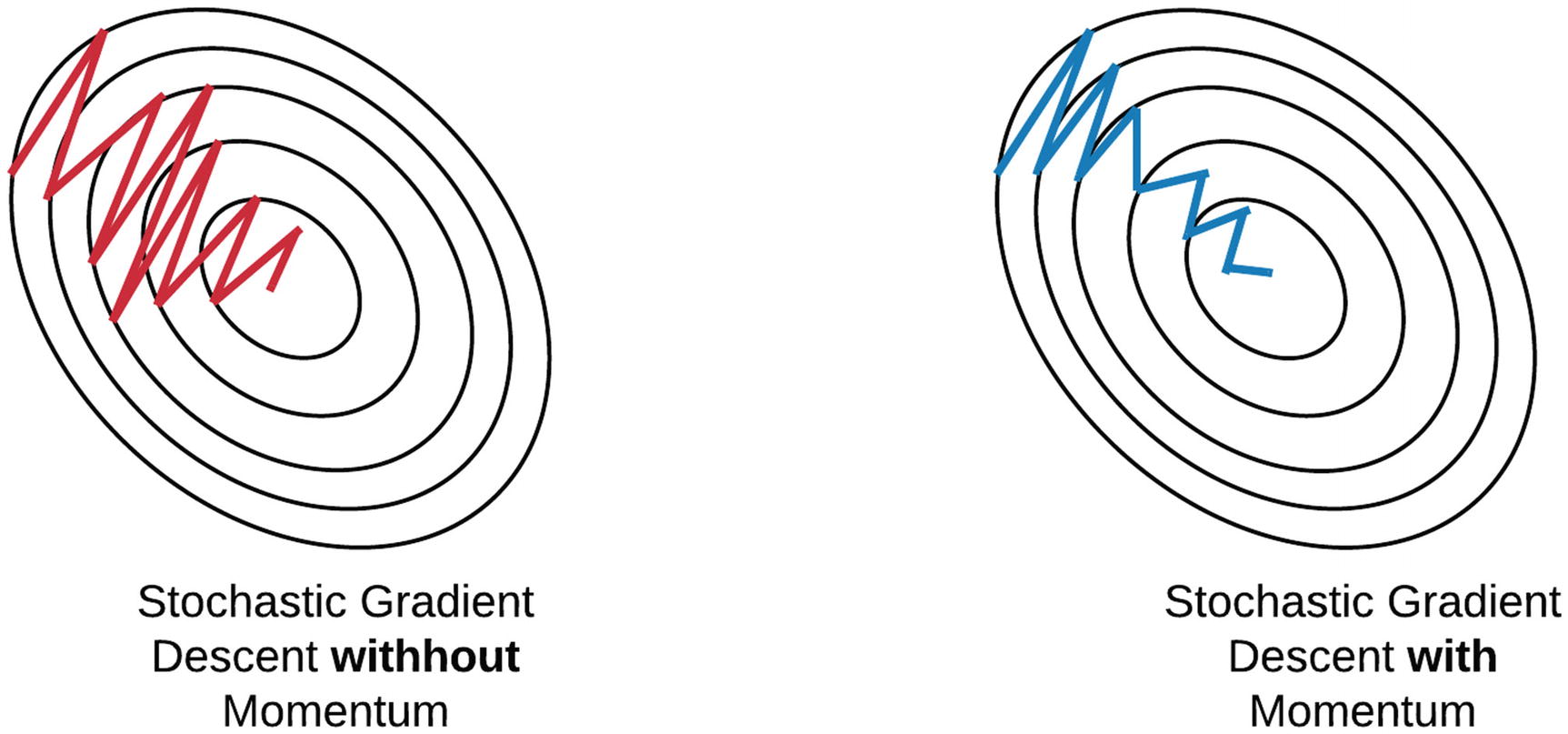
There are many ways ...

There are many way and forms of momentum. Pytorch implementation is different from other frameworks and Nesterov momentum.

$$v_{k+1} = \mu v_k + g_{k+1}, \quad p_{k+1} = p_k - \alpha \cdot v_{k+1}.$$

Sutskever paper in 2013 proposed

$$v_{k+1} = \mu v_k + \alpha \cdot g_{k+1}, \quad p_{k+1} = p_k - v_{k+1}.$$

The initial idea of momentum has been proposed by Y. Nesterov in 1983 for convex tasks.

$$\phi_{k+1} = \theta_k - \alpha_k \nabla_{\theta} g(\theta), \quad \theta_{k+1} = \theta_k - \mu_k (\phi_{k+1} - \phi_k).$$

NAG has been shown to be optimal for convex functions.

Adaptive gradient

Duchi et. al 2011 introduced Adagrad.

The overall formula is typically written as

$$\theta_{k+1} = \theta_k - \alpha \mathrm{diag}(\varepsilon I + G_k)^{-1/2} g_k,$$$$G_k = \sum_{s=1}^k g_s g^{\top}_s.$$

Basically, we estimate very roughly the correlation between gradients and try to decorrelate it

One can replace averaging with exponential weighted average (AdaDelta).

Adam

Adam is superpopular optimization method and a method of choice for training many DNN.

$m_{k+1} = \beta_1 m_k + (1-\beta_1) g_k$

$v_{k+1} = \beta_2 v_k + (1-\beta_2) g_k^2$

$\hat{m}_{k+1} = \frac{m_{k+1}}{1-\beta_1^{k+1}}$

$\hat{v}_{k+1} = \frac{v_{k+1}}{1-\beta_2^{k+1}}$

$\theta_{k+1} = \theta_k - \frac{\eta}{\sqrt{\hat{v}_{k+1}}+\epsilon} \hat{m}_{k+1}$

where $m_k$ and $v_k$ are the first and second moment estimates of the gradients up to iteration $k$, $\beta_1$ and $\beta_2$ are the exponential decay rates for the moment estimates, $\hat{m}_{k+1}$ and $\hat{v}_{k+1}$ are bias-corrected moment estimates, and $\epsilon$ is a small constant to prevent division by zero. The Adam optimizer combines the benefits of momentum and adaptive learning rates to achieve faster convergence and better generalization.

Fun facts: There exist examples where vanilla Adam does not converge. There are some (not very popular) alternatives.

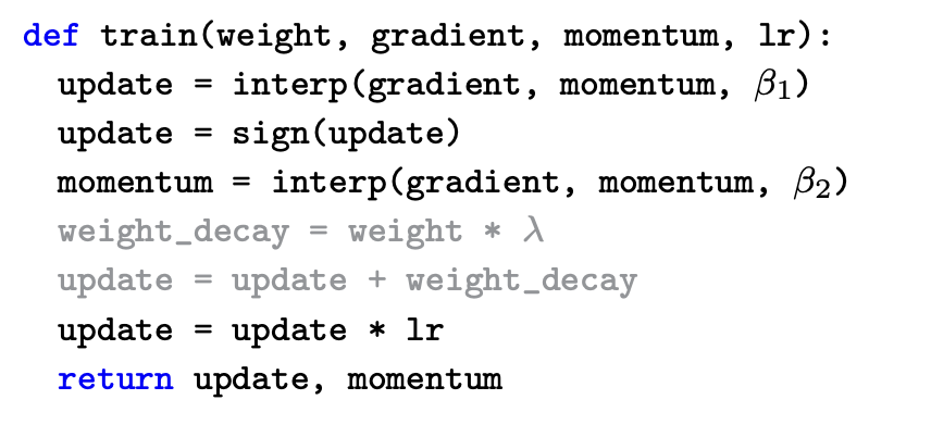
Recent: LION optimizer

Symbolic Discovery of Optimization Algorithms

A very smart search through all possible algorithms using genetic algorithms (here interp is just convex combination with parameter). Note, that only the sign of the update is used.

Comparison of optimization methods with advantages and disadvantages

• All of the standard methods are compatible if properly tuned.
• In practice, people use learning rate scheduling of different types
• SGD is much more sensitive to it, can generalize better
• SGD has less memory (2 vectors stored vs 3 for Adam), but it can be remedied.

No systematic analysis for non-convex case, almost systematic in the convex case.

Very interesting models for the noise and the effect of clipping (present in Adam, see work by Gasnikov et. al.).

Potentially, this could be an explanation why Adam-type method works.

Explanation of the problems with training deep models

Vanishing Gradients and Catastrophic Forgetting

Vanishing gradients: when gradients become very small and slow down learning

• Vanishing gradients is a phenomenon that occurs in deep neural networks during training.
• It happens when the gradients of the loss function with respect to the weights and biases of the lower layers become very small.
• This can happen because the gradients are multiplied by the weights of each layer during backpropagation, and if these weights are small, the gradients can become exponentially smaller as they propagate through the network.
• The lower layers of the network may not receive enough information to update their parameters effectively, which can lead to slow or ineffective training.
• Vanishing gradients can be mitigated by using activation functions that have non-zero derivatives, initializing the weights carefully, or using techniques such as batch normalization or residual connections.

Importance of normalization in deep neural networks

One of the important techniques to tackle the problem of vanishing gradients are normalization layers.

The first layer has been Batch Normalization

Batch Normalization

Let $x$ be minibatch,

$$\mathrm{BN}(\mathbf{x}) = \boldsymbol{\gamma} \odot \frac{\mathbf{x} - \hat{\boldsymbol{\mu}}_\mathcal{B}}{\hat{\boldsymbol{\sigma}}_\mathcal{B}} + \boldsymbol{\beta}.$$

Here $\hat{\boldsymbol{\mu}}$ are sample mean and $\hat{\boldsymbol{\sigma}}$, respectively for the minibatch.

Batch Normalization: details

For FC layers, apply the scheme described above;

For convolutional layers, store one mean and one variance for a channel (for pure convolutional networks it is useful because we can use for different size).

On the inference and train, the models are evaluated in a different way.

We compute the sample mean and variance over entire dataset and fix them, i.e. BN is now just a simple linear transformation.

Layer Normalization

For convolutional layers, BN is defined even of batch size = 1.

This lead to the development of layer normalization, which is defined as

$$\mathbf{x} \rightarrow \mathrm{LN}(\mathbf{x}) = \frac{\mathbf{x} - \hat{\mu}}{\hat\sigma},$$$$\hat{\mu} \stackrel{\mathrm{def}}{=} \frac{1}{n} \sum_{i=1}^n x_i \text{ and } \hat{\sigma}^2 \stackrel{\mathrm{def}}{=} \frac{1}{n} \sum_{i=1}^n (x_i - \hat{\mu})^2 + \epsilon.$$

We just make the mean value and variance accross activations (not batch) equal to $0$ and $1$, respectively.

Instance Normalization

Proposed by D. Ulyanov et. al:

This prevents instance-specific mean and covariance shift simplifying the learning process. Intuitively, the normalization process allows to remove instance-specific contrast information from the content image in a task like image stylization, which simplifies generation.

$$y_{tijk} = \frac{x_{tijk} - \mu_{ti}}{\sqrt{\sigma_{ti}^2 + \epsilon}}, \quad \mu_{ti} = \frac{1}{HW}\sum_{l=1}^W \sum_{m=1}^H x_{tilm}, \quad \sigma_{ti}^2 = \frac{1}{HW}\sum_{l=1}^W \sum_{m=1}^H (x_{tilm} - \mu_{ti})^2.$$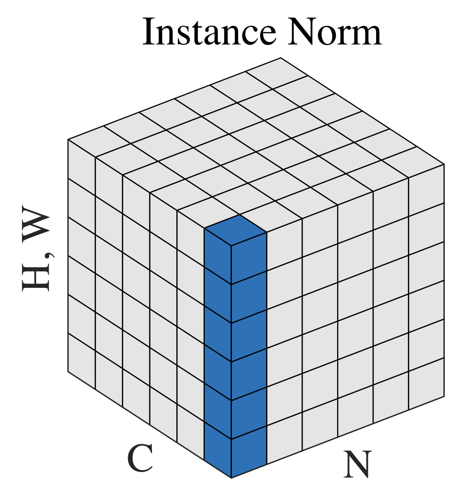

Catastrophic forgetting: when a model forgets previously learned information when learning new information

• Catastrophic forgetting is a phenomenon that occurs in machine learning models, particularly in neural networks, where the model forgets previously learned information when it is trained on new data. T
• This happens because the model updates its weights and biases based on the new data, which can cause it to overwrite the previously learned information.

(Practical) solutions

In practice, people can do the following:

• Train on the new data and sometimes mix the old data in (for example, mixing the gradients with some weights)
• Another solution is just to add regularization to the distance between new and old weights.
• Could be actually important in such tasks as distillation.

Techniques to mitigate these problems, such as skip connections and continual learning

Importance of initialization in deep neural networks

In optimization, we need to initialize the parameters at the start.

If we initialize badly, we may have vanishing gradients in the beginning.

Typically, weights have been initialized to uniform or Gaussians.

Glorot and Bengio proposed to scale the initial distributions to get better results (2016)

Idea of initialization

Suppose we have a linear network

$$y = W_L \ldots W_1 x.$$

Then, we would like to have the mean and variance after one multiplication.

We can initialize bias to $0$ and $W_i$ to be $N(0, \sigma_i)$, $\sigma_i \sim \frac{1}{n_i}$, where $n_i$ is the width of the $i$-th layer.

This method works well for activation functions which have linear region around $0$, i.e. tanh activations.

For ReLU you have to use different method.

He initialization

He initialization involves setting the initial weights to random values drawn from a normal distribution with mean 0 and variance $\frac{2}{n_{in}}$, where $n_{in}$ is the number of input connections to the layer. The formula for He initialization can be written as:

$$W \sim \mathcal{N}(0, \frac{2}{n_{in}})$$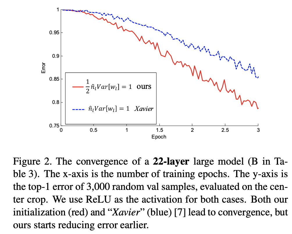

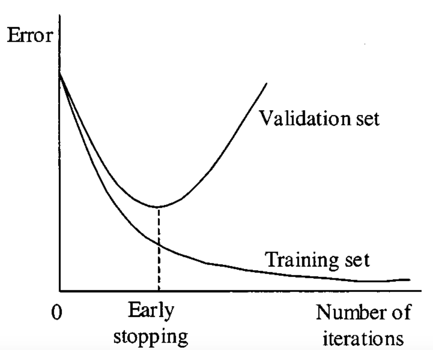
Early Stopping

Deep learning may overfit too much.

Thus, besides train and test it is important to dedicate some samples to the validation set and monitor the convergence on it, and stop if it is starting to grow.

Loss Surfaces

Do we understand why the methods work and how they converge?

Short answer: No.

We can visualize the minima:

• Understanding Generalization through Visualizations

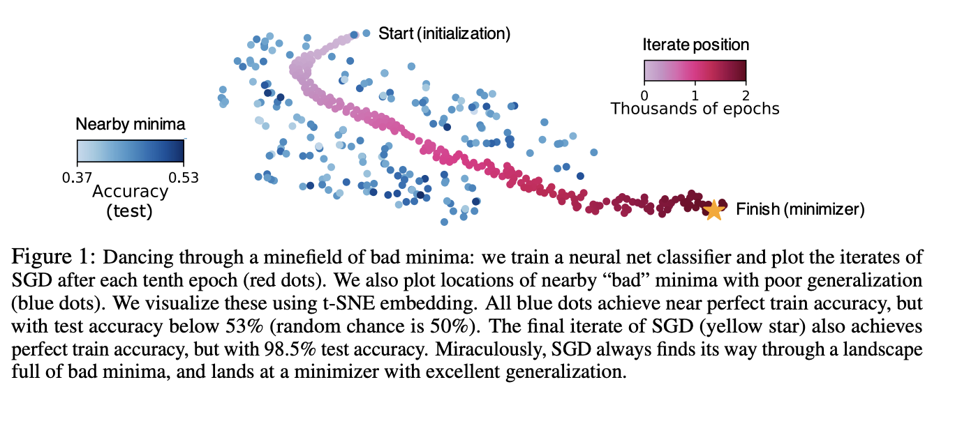
Common hypothesis

SGD finds wider minima (easy to believe under certain assumptions), which generalize better (not clear).

You can formulate many interesting experiments to do that will be counter-intuitive.

Some more advanced facts: the distribution of noise in SGD is different for CNN and transformer models.

Double descent phenomena

A systematically observed phenomena for training larger models. The convergence has three stages: classical, interpolation, and then modern regime.

M. Belkin has analyzed this for kernel-type methods.

Take home message

• SGD optimization methods (SGD with momentum, Adam, ...)
• Problems with training deep models: vanishing gradients, catastrophic forgetting
• Effect of initializations
• Normalizations
• Early stopping
• Interesting properties of loss surfaces of DNN models

Next lecture: СV tasks

• object detection
• semantic segmentation
• transfer learning