Lecture 4: СV tasks
Previous lecture: Training better
- SGD optimization methods (SGD with momentum, Adam, ...)
- Problems with training deep models: vanishing gradients, catastrophic forgetting
- Effect of initializations
- Normalizations
- Early stopping
- Interesting properties of loss surfaces of DNN models
Todays lecture
- object detection
- semantic segmentation
The most popular CV tasks
The most popular computer vision (CV) task is classification.
We already discussed the supervised learning setting, loss functions (we put softmax to predict probabilities),
and we train them on large datasets using SGD-type methods
(with actually a lot of tricks which we will discuss later, both to improve generalization and computational efficiency)
Basic architectures were also discussed before (CNN, ResNet).
Visual Transformer models will be discussed later in this course.
Brief reminder: evaluation metrics for classification tasks, accuracy, precision, recall
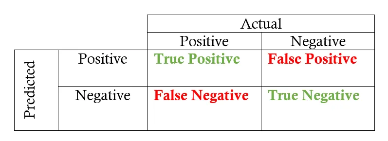
Typically, we talk about accuracy (percentage of correct predictions). Works well when classes are balanced (i.e. have similar number of samples).
Accuracy: $$A = \frac{TP+TN}{TP+FP+TN+FN}.$$ Precision $$P = \frac{TP}{TP+FP}.$$ Recall $$R = \frac{TP}{TP+FN}.$$ F1 score (harmonic mean between precision and recall) $$F1 = 2 \frac{R \circ P}{P + R}.$$
Finally, ROC (Receiver operating curve) is a plot between True Positive rate (TPR = Recall) and False Positive Rate (FPR),
$FPR = \frac{FP}{TN+FP}.$
We change the threshold between positive class and negative class. AUC is the area under the curve. We want to make it bigger.
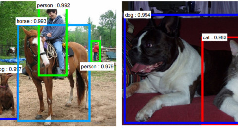
Object detection.
The goal of object detection is (!) detect objects on images. The detection includes:
- the detection of the bounding box of the object.
- the detection of the class of the object.
Applications of object detection
- Number 1: FaceID systems use face detection module in the first place
- Autonomous driving
- Medical applications
- Robotics
How the data looks like.
There are quite a lot of datasets for object detection, see paperswithcode
- Subset of imageNet has object locations (i.e. multiple objects in the same photo, approximately 3 per image, in total 1,034,908 images, see paperswithcode).
- MS Coco dataset
- Smaller (kind of 'MNIST' is Pascal VOC.
- Not too many new ones (probably superseeded by semantic segmentation as more complex task, I am not actually sure why).
How we evaluate object detection models
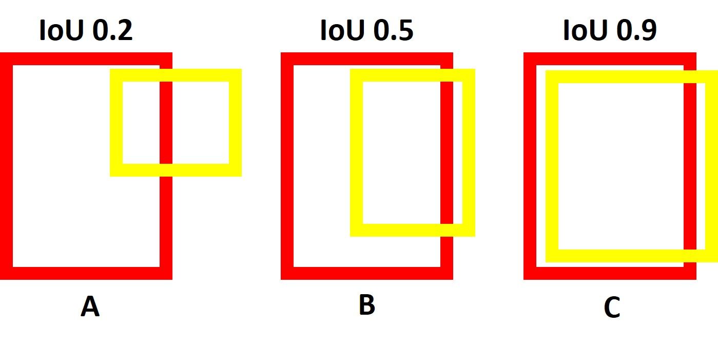
The prediction of the boxes is measured using IoU measure.
The prediction of the classes is computed using mean average precision (mAP) measure:
The reason is that we can have different classes in one image, and different thresholds have to be used.
Average precision
In order to compute average precision (for object detection), we compute precision-recall curve for different threshold, i.e. if $IoU > t$ the class is positive, if this is not satisfied -- the class is negative.
Once precision and recall values are computed, we compute
$$AP = \sum_{k=0}^{k-n} [R(k)-R(k+1)] P(k),$$which is just the area under the curve for precision-recall. AP is always between 0 and 1 (check!)
In object detection we have different classes, and they can use different thresholds!
We just average AP for different classes and thats all!
This is a standard metric for benchmarking object detection.
Architectures
Bunch of successful classical detectors (Viola-Jones, SIFT/Hog, used for face detection mainly)
First succesfull CNN architecture has been R-CNN architecture.
R-CNN stands for region proposal CNN
YOLO (You look only once) model family
Modern: transformer-based models
R-CNN
The original R-CNN has the flavour of classical methods.
First, the authors used selective search (which looks at things like histograms to measure the similarity between regions) to select large number (2000) of candidates.
Then, these regions are warped into a square and fed into a CNN which generates a vector of dimension 4096.
The extracted features are fed into SVM to classify if the object is in the region or not.
The algorithm also predicts the offset values (4 of them) for the object bounding box.
Problems with R-CNN
- Fixed selective search algorithm
- Very long training
- Inference is not real time.
Next step: Fast R-CNN
In the fast R-CNN model:
- Do the CNN first
- Do selection search on features (still you see it here, authors did not believe you can get rid of it or they really liked it!)
- Since convolution has limited reception field, the original objects are mapped to some (bounded) objects in the feature map
- Faster than R-CNN and slightly more accurate
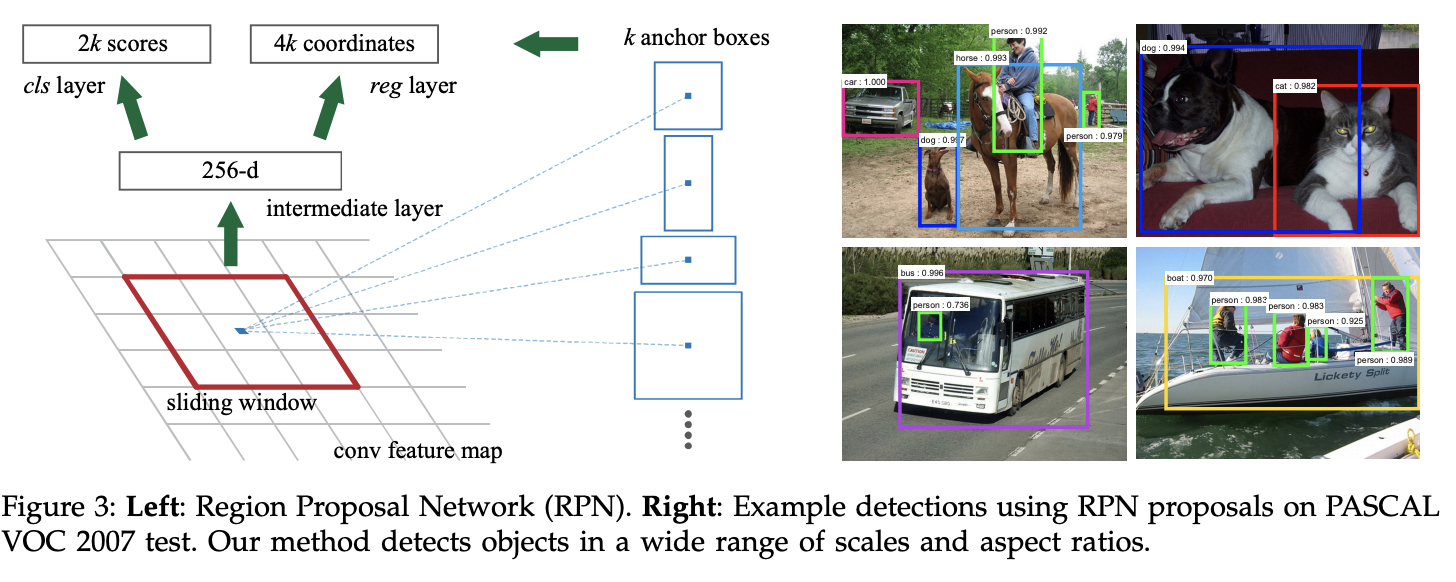
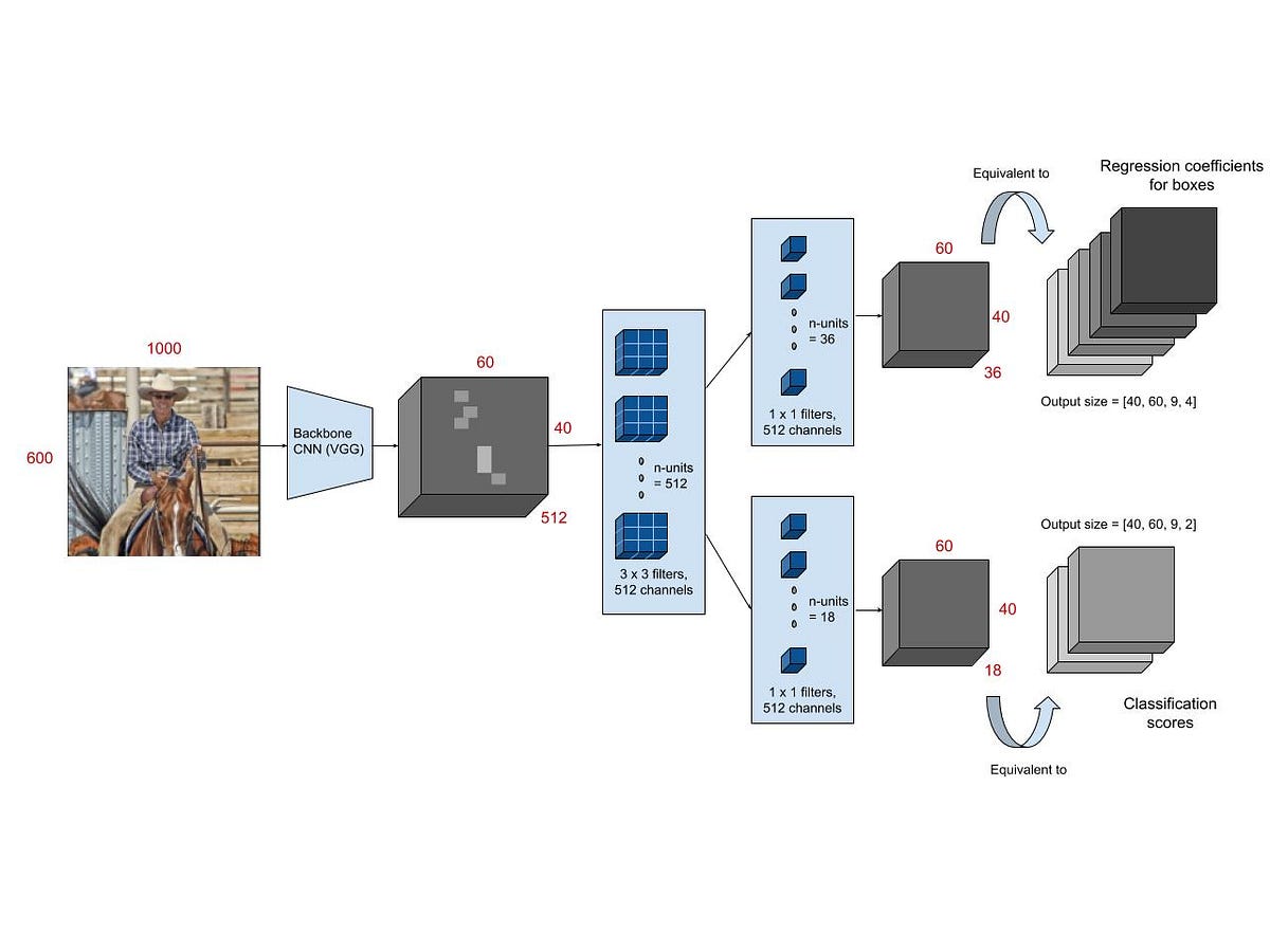
Next step(2): Faster R-CNN
- Key idea was to replace the selective search algorithm by another neural network that predicts the region.
- The layer is region proposal network
- The loss is classification (for object) and regression (for boundaries).
- ROI pooling layer
Summary of R-CNN family
The Faster R-CNN has become much faster (more than 100x) and could be used for real-time detection.
You can change backbones as well to more modern architectures easily!
YOLO models
In R-CNN models, neural networks first look for regions where the object can be located and works with the regions.
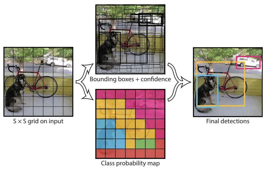
In YOLO (You look only once) a single CNN predicts the bounding boxes and classes simultaneously
The input is split into $S \times S$ grid.
For each cell we predict $B$ bounding boxes. Each box is $(x, y, w, h, confidence)$. The grid prediction is done through the size of the output tensor, which is $S \times S \times (5 B + C)$.
Differences between YOLO and R-CNN
- YOLO is much faster
- YOLO looks globally at the image in a single CNN.
YOLOv2
In YOLOv2 several improvements have been made:
- Different backbone based on VGG
- Anchor boxes (predefined boxes of different size + predicted BB).
- Batch normalization
Faster and more accurate!
Next generations of YOLO
- 2016: YOLOv3 ResNet architecture (called Darknet-53) and Feature Pyramid networks.
- 2018: YOLOv4 (developed not by original team): new architecture (called CSPNet, based on DenseNet) + new loss (to improve on imbalanced datasets).
- 2020: YOLOv5 (developed by original team) -- EfficientDet (based on EfficientNet).
- 2022: YOLOv6, new backbone + new method for anchor prediction.
- 2023: YOLOv7: focal loss $FL(p_t) = (1-p_t)^{\gamma} \log p_t$, putting more weight on missclassified examples.
VIT
As a backbone, you can also use vision transformers as a backbone(will discuss if time permits and I will not forget to do it).
Summary of this part
- There are different families for efficient object detection (R-CNN & YOLO).
- They do have some problems, but overall the quality is growing due to extensive engineering efforts
- The dataset collection is also important.
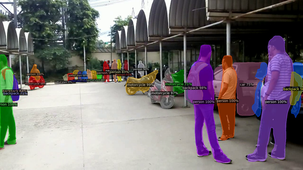
Image segmentation
There are several types of image segmentation.
That includes:
- Semantic segmentation (every pixel belongs to a specific data)
- Instance segmentation (separation of the image into regions with classes)
- Panoptic segmentation (predicts the identity of each object)
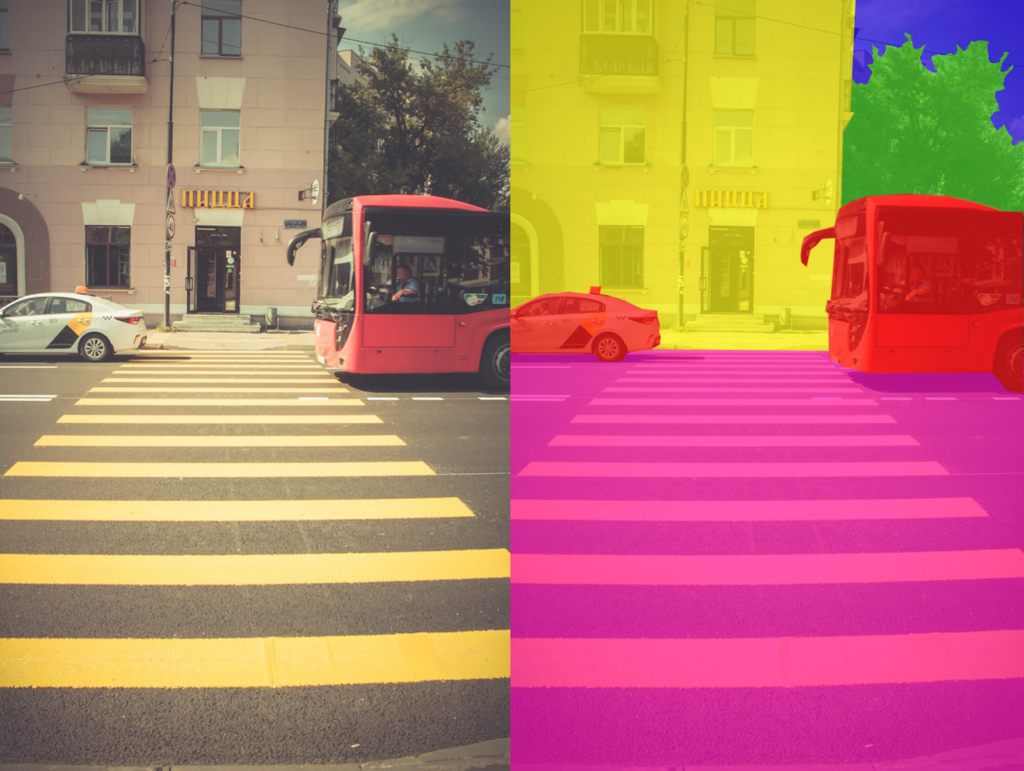
Semantic segmentation
In semantic segmentation, we need to predict the class of each pixel (i.e. all trees, all persons, etc.). This is an example of image-to-image transformation: as an input, we have an image, as the output we have the mask
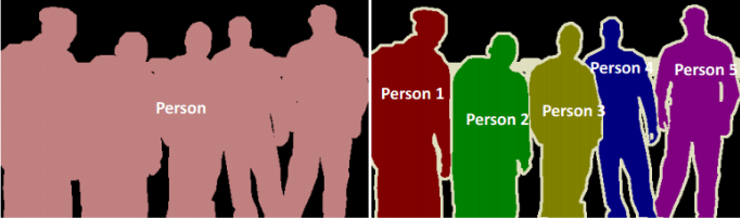
Instance segmentation
In instance segmentation, we need to predict not only the class, but also the instances of the object.
Similar to object detection, but
Panoptic segmentation
Panoptic segmentation combines best of both worlds.
Each pixel in a scene is assigned a semantic label
(due to semantic segmentation) and a unique instance identifier (due to instance segmentation).
Evaluation metrics for image segmentation
- IoU (already covered) for semantic segmentation
- Instance segmentation is measured using average precision
- Panoptic uses Panoptic Quality which evaluates the predicted masks and instance identifiers. PQ unifies evaluation over all classes by multiplying segmentation quality (SQ) and recognition quality (RQ) terms. SQ represents the average IoU score of the matched segments, while RQ is the F1 score calculated using the precision and recall values of the predicted masks.
- DICE coefficient which is simply two times the overlap area divided by the total number of pixels in both images
Architectures for semantic segmentation
There are quite a few architectures for semantic segmentation including:
- SegNet
- U-Net
- FCNs
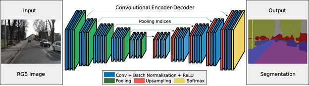
SegNet
SegNet was the first architecture and had the following form of the image-to-image (pix2pix) architecture
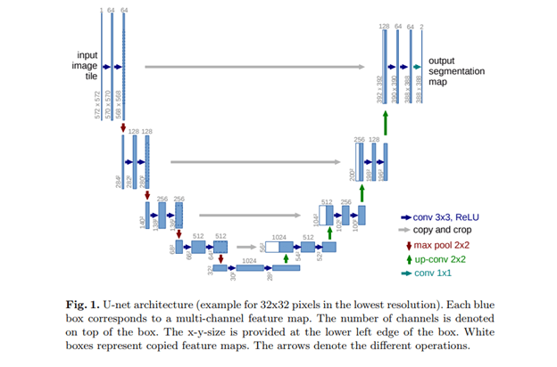
U-Net
U-Net is still one of the most popular architectures for image-to-image models and is used in diffusion models.
The key idea is to add skip connections to ensure multiscale processing of the input data.
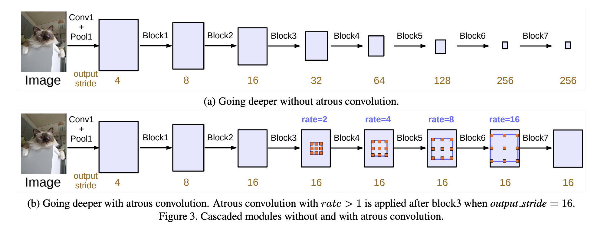
Dilated convolutions
Several backbones (DeepLab v.1,2, 3) use dilated (atrous) convolutions to build the encoder, for example https://arxiv.org/pdf/1706.05587v3.pdf
These convolutions replace pooling, which is good for abstract features but not for pixel predictions
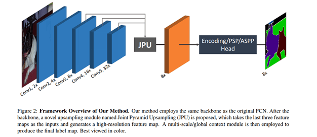
FastFCN
A Fast Fully Convolutional network based on DeepLabv3 is used to replace dilated convolutions (which take a lot memory and time). The original FCN paper uses upsampling with dilated convolutions The fast version takes the last 3 conv layers and uses Joint Pyramid Upsampling from those layers.
Losses for image segmentation
There are quite a lot of different losses for the segmentation problems, see review
| Type | Loss Function |
|---|---|
| Distribution-based Loss | Binary Cross-Entropy |
| Weighted Cross-Entropy | |
| Balanced Cross-Entropy | |
| Focal Loss | |
| Distance map derived loss penalty term | |
| Region-based Loss | Dice Loss |
| Sensitivity-Specificity Loss | |
| Tversky Loss | |
| Focal Tversky Loss | |
| Log-Cosh Dice Loss | |
| Boundary-based Loss | Hausdorff Distance loss |
| Shape aware loss | |
| Compounded Loss | Combo Loss |
| Exponential Logarithmic Loss. |
Losses for segmentation
Since segmentation can be viewed as classification, the distribution-based losses (including the focal loss) are clear.
One can also use the differentiable version of the Dice loss, defined as
$$DL(y, \hat{p}) = 1 - \frac{2 y \hat{y} + 1}{y + \hat{y}+1}$$It is claimed that it works better for imbalanced datasets (typically, medical data).
Many other losses and a lot of engineering!
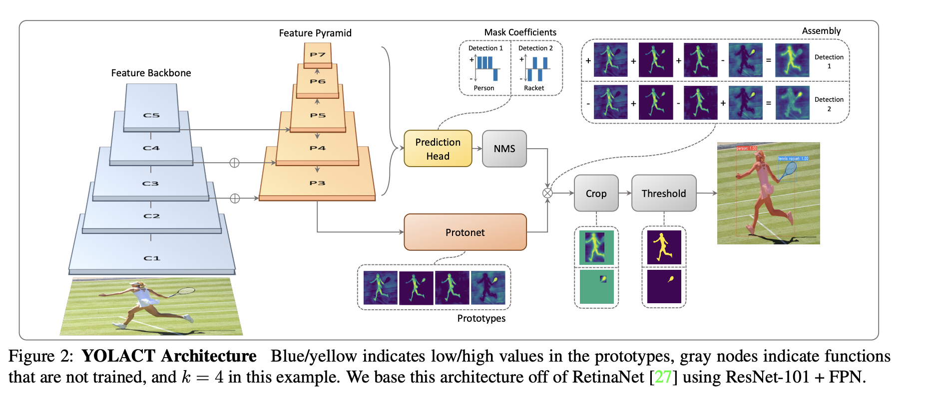
Architectures for instance segmentation
Not lets discuss Instance Segmentation. Some of the popular architectures include:
- Mask R-CNN
- PANet
- YOLACT
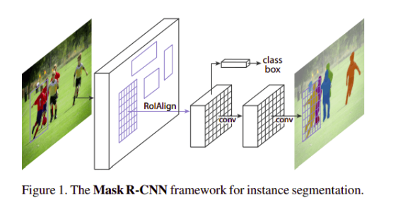
Mask R-CNN
Mask-R-CNN (Detectron by Facebook, now Detectron2.
The difference with Detectron and Detectron2 is that the latter is written in Pytorch, includes panoptic segmentation and DensePose.
The original architecture is extension of Faster R-CNN described before.
The model generates the bounding box and segmentation for each instance.
Addinal head that predicts the mask!
The total loss will be a sum of three losses (class, box, mask).
RoI Align solves the problem of different size of the feature map and the region map by using interpolation (we have to fit a part of the feature map to a known region).
PANET
PANET architecture studies a practical case of few shot image segmentation.
We will talk about zero-shot/few-shot architectures later on in the course.
The idea is that we only have few examples per class.
Details later on! (Remind me if I forget about it, since it is useful to explain few-shot classification before few-shot segmentation!).
Summary
- Object detection
- Image segmentation
- I probably missed a lot, so stay tuned (if not) for CV courses!
Next lecture: Learning from sequential data
- Recurrent neural networks and their variants (RNN, GRU, LSTM).
- The concept of attention
- Transformer models