Lecture 5: Modelling sequences
Previous lecture: CV tasks
- object detection (R-CNN, YOLO), metrics for evaluation
- semantic segmentation (Masked R-CNN, U-Net), instance segmentation
Todays lecture
- Modelling sequences
- Recurrent neural networks (RNN) and their variants: RNN, GRU, LSTM
- Concept of attention
- Transformer architecture
Modelling sequential data
Suppose we have (discrete) sequence as a single sample:
$$x_1, \ldots, x_T$$Examples:
- Natural Language Processing (NLP), where $x_i$ are discrete tokens
- Time series of different kinds (sensor data, EEG data, ...)
We need to have (deep) architectures that process sequential data in order to solve different downstream tasks
Recurrent neural networks
The difference between MLP and Recurrent Neural Networks (RNN) is that it should be able to process sequences of different length.
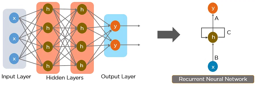
Types of RNN
In simple RNN, we introduce a hidden state and process the input using 1 layer:
Elman network:
$$h_t = \sigma(W_h x_t + U_h h_{t-1} + b), \quad y_t = \sigma(W_y h_t + b_y).$$Jordan network:
$$h_t = \sigma_h(W_h x_t + U_h y_{t-1} + b), \quad y_t = \sigma_y(W_y h_t + b_y).$$Questions
$$h_t = \sigma(W_h h_t x_t + U_h h_{t-1} + b), \quad y_t = \sigma(W_y h_t + b_y).$$Suppose we want to solve classification tasks
How do we train the model?
What are possible problems?
Training using unfolding
If we make $k$ steps, we can represent the resulting code a DNN with $k$ layers.
This process is called unrolling.
We can then differentiate through it in a normal way.
The problems are standard: although we have to learn few parameters, the gradients can vanish.
One of the breakthrough solutions have been long short-term memory model.
Vanishing gradients
Since the computational block of RNN is the same, the Jacobians are the same.
The gradient in backpropagation will have the form $$W^k v$$.
So, if the eigenvalues of $W$ are less than $1$ we get exponential decay.
If the eigenvalues are greater than $1$, we get exponential growth.
If they are one (for example for orthogonal weight matrices) you can get much more stable training of RNN.
(That is why orthogonal parametrization can be important!)
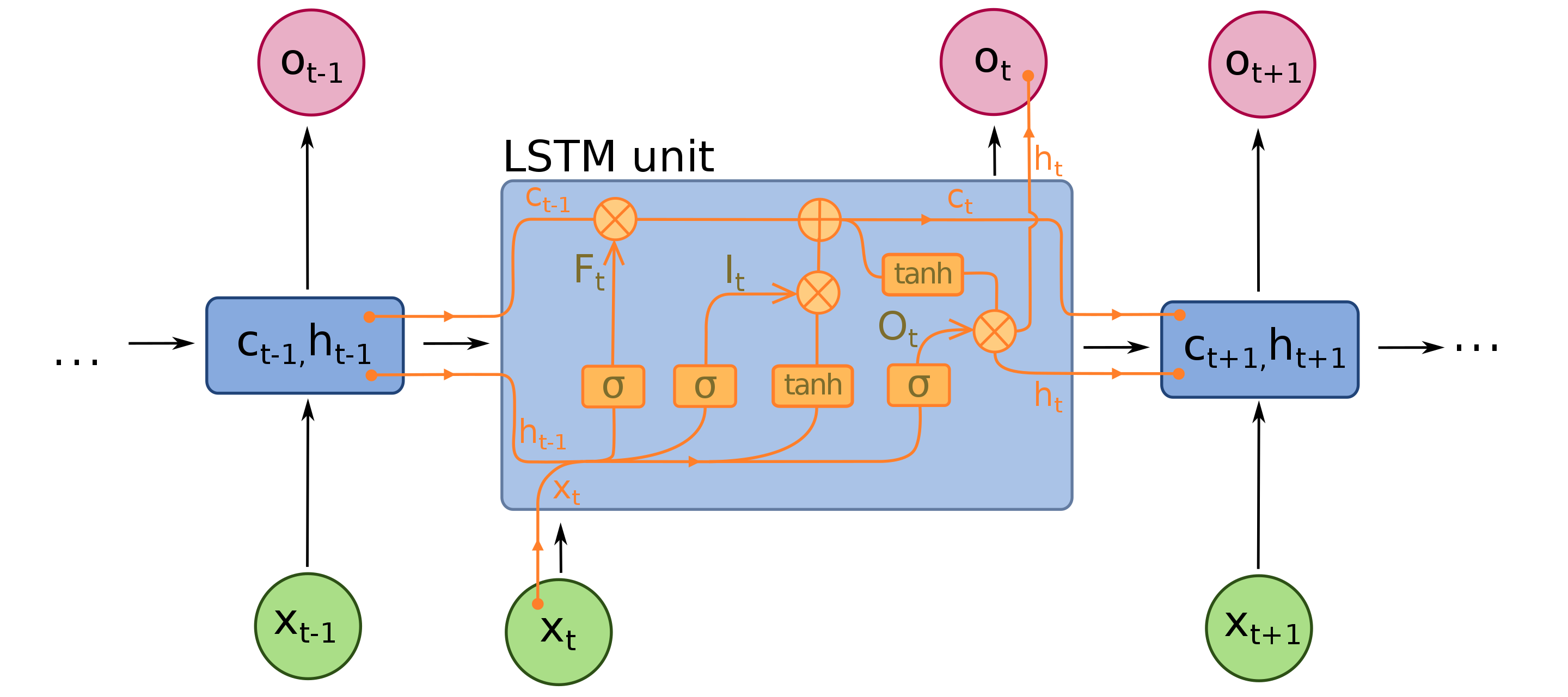
LSTM: introducing memory
The LSTM unit has the following multiplicative gating mechanism
\begin{align} f_t &= \sigma(W_f[x_t, h_{t-1}] + b_f) \\ i_t &= \sigma(W_i[x_t, h_{t-1}] + b_i) \\ \tilde{C}_t &= \tanh(W_C[x_t, h_{t-1}] + b_C) \\ C_t &= f_t \odot C_{t-1} + i_t \odot \tilde{C}_t \\ o_t &= \sigma(W_o[x_t, h_{t-1}] + b_o) \\ h_t &= o_t \odot \tanh(C_t) \end{align}where:
- $x_t$ is the input at time step $t$
- $h_{t-1}$ is the hidden state at time step $t-1$
- $f_t$, $i_t$, $o_t$ are the forget gate, input gate, and output gate vectors respectively
- $\tilde{C}_t$ is the cell input vector
- $C_t$ is the cell state at time step $t$
- $\odot$ represents element-wise multiplication
- $\sigma$ is the sigmoid activation function
- $W_f$, $W_i$, $W_C$, $W_o$ are weight matrices for each gate and cell input
- $b_f$, $b_i$, $b_C$, $b_o$ are bias vectors for each gate and cell input.
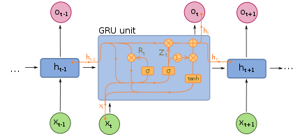
Gated recurrent unit
GRU (Gated recurrent unit) is a simpler version of LSTM that has been introduced in 2014. It shows similar performancce.
\begin{align} r_t &= \sigma(W_r[x_t, h_{t-1}] + b_r) \\ z_t &= \sigma(W_z[x_t, h_{t-1}] + b_z) \\ \tilde{h}_t &= \tanh(W_h[x_t, r_t \odot h_{t-1}] + b_h) \\ h_t &= (1 - z_t) \odot h_{t-1} + z_t \odot \tilde{h}_t \end{align}where:
- $x_t$ is the input at time step $t$
- $h_{t-1}$ is the hidden state at time step $t-1$
- $r_t$ and $z_t$ are the reset gate and update gate vectors respectively
- $\tilde{h}_t$ is the candidate activation vector
- $h_t$ is the updated hidden state at time step $t$
- $\odot$ represents element-wise multiplication
- $\sigma$ is the sigmoid activation function
- $W_r$, $W_z$, $W_h$ are weight matrices for each gate and candidate activation
- $b_r$, $b_z$, $b_h$ are bias vectors for each gate and candidate activation.
Other types of RNN
- Bi-direction RNN
- Second-order RNN
- More complexicated neural networks as a building blocks
How to train RNN-type models.
One of the main challenges in sequence modelling is to predict the next symbol (vector) in the sequence.
Extrapolation or prediction is one of the most important and challenging tasks.
This can be viewed as seq2seq problem: given $x_1, \ldots, x_T$ we want a model to output $x_2, \ldots, x_{T+1}$.
A widely used loss in this context is Connectionist temporal classification (CTC) loss.
CTC loss
CTC loss is quite complicated loss, if we need to map a sequence of one length to the sequence of another length. We add additional 'blank' symbol as an output, use softmax to process RNN/LSTM data and need to compute the sum over all possible alignments.
There a lot of alignments, so dynamic programming needs to be used.
$$\mathcal{L}_{\text{CTC}}=-\sum_{\pi \in \mathcal{B}(y)}p(\pi|x)$$where:
- $\mathcal{L}_{\text{CTC}}$ is the CTC loss
- $\mathcal{B}(y)$ is the set of all possible alignments of the target sequence $y$
- $p(\pi|x)$ is the probability of alignment $\pi$ given the input sequence $x$.
Concept of attention
When processing the sequence, all the information about the previous states is summarized in the hidden state.
This may not be enough, and we want to have an opportunity to look at the previous elements in the sequence when we need it.
A natural idea is to consider similar patterns in the sequence, which might help prediction.
Of course, we can just use extended history, but it is typically not enough.
Concept of attention (2)
Attention has been first introduced in 2015 in the paper by Bengio et. al on Neural Nachine Translation
The attention weights were a function
$$e_{tj} = a(h_t, s_{t-1}), \quad \alpha_{tj} = \frac{\exp(e_{tj})}{\sum_{k=1}^T \exp(e_{tk})}$$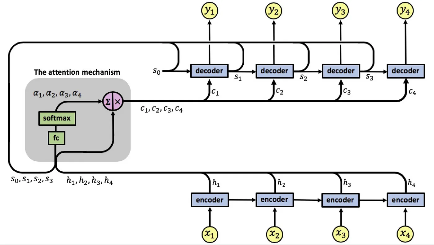
Attention is all you need
A seminar paper has been attention is all you need which greatly simplified original architecture of RNN-type models with attention and also introduced the concept of self-attention.
In self-attention, we start from a sequence $X$ parametrized by a matrix of size $N_{seq} \times N_{f}$, where $N_{seq}$ is the length of the sequence, and $N_f$ is the dimension of the vector space representing the sequence.
We need to compute similarities between the vectors in the sequence.
To do so, we map $X$ to query and key values by using linear transformations:
$$Q = X W_Q, K = X W_K.$$The similarity between the $i$-th element of the sequence and the $j$-th element of the sequence is then given as a scalar product between corresponding columns:
$$\hat{M}_{ij} = (q_i, k_j).$$In order to make these attention weights, we use softmax operation along the columns, so
$$M = \mathrm{softmax}\left({\frac{QK^{\top}}{\sqrt{d_k}}}\right).$$The attention matrix has the properties $M_{ij} \geq 0, \sum_j M_{ij} = 1$.
Self-attention
In self-attention block, the input sequence $X$ is being mapped to three matrices $Q, K, V$ (called query, key and value) and the transformation of $X$ to the output is given by
$$Q = X W_Q, \, K = X W_K, \, V = X W_V.$$$$\mathrm{Attention(Q, K, V)} = \mathrm{softmax}\left({\frac{QK^{\top}}{\sqrt{d_k}}}\right) V,$$which is just taking linear combinations of vectors in $V$ with the attention weights.
Designing the transformer model
The attention block allows us to exchange information between each component of a sequence.
Then, we can process the information along the feature dimension using MLP.
Originally, people tried to use convolution, but ended up using MLP, but in some of the code historically we have Conv1D block.
Also, we use not one attention head, but many of smaller dimensions.
If we have H heads, we compute $H$ attention matrices.
The resulting output has the same size, since $Q_i, K_i$ have smaller number of rows.
Thus, we use multihead attention (why?) and feedforward MLP to process the features.
Comments
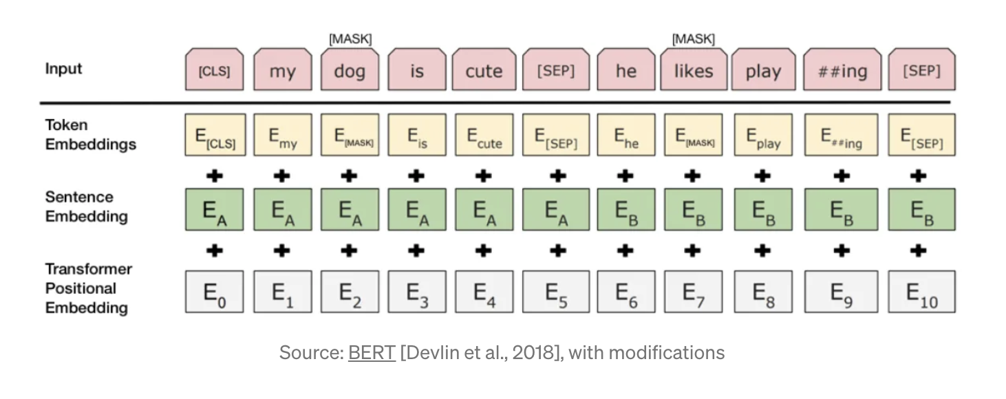
- The architecture starts from the embedding block. Since the main application of transformers is NLP, we map discrete sequence elements from the vocabulary to the embedding vectors.
- We also use positional encoding: i.e., without it the result will be invariant to permuations. The positional encoding is added to each embedding vectors. There are many types of positional encoding.
- A transformer block contains: a) multihead attention b) MLP block
- MLP block has two feedforward layers. The first one increases the dimension by a factor of $4$, then second one brings the dimension down, i.e. this is a reversed bottleneck block. It also has skip-connections and layer normalization.
- We repeat the blocks as many times as we want.
- The parameters of the transformer model are number of blocks, number of heads, the dimension of embedding.
Training transformer models
For seq2seq (encoder-decoder models) we can just convert the embeddings to the probabilities of the symbol and then maximize the likelihood of the sequence.
However, one of the most important applications of transformer models is unsupervised learning: we do not have any parallel corpus.
Lets decribe the GPT (Generalized pretrained transformer) model.
GPT model
In GPT model, we have the data, which each sample being a sequence $x_1, \ldots, x_T$. We want to learn the probability distribution
$$p(x_1, \ldots, x_T)$$We parametrize this distribution in the autoregressive form (typically it is referred to as autoregressive language modelling)
$$p(x_1, \ldots, x_T) = p(x_1) p(x_2 \vert x_1) p(x_3 \vert x_1, x_2) \ldots, $$i.e. we want to learn conditional probabilities of the next symbol given all the previous ones.
This gives the standard objective of the GPT: predict the probability of the next symbol given all the previous ones.
Predicting probabilities of the next symbol
For the efficient training, we parametrize all conditional probabilities using a single Transformer model.
We process the input data $x_1, \ldots, x_T$ by several transformer layers, get embeddings $h_1, \ldots, h_T$.
We use masked attention: at each self-attention step we multiply the mask by a matrix $L$, where
$$L_{ij} = \begin{cases} 1, \quad i \geq j, \\ 0, \mbox{otherwise}\end{cases}.$$This means, that the $j$-th embedding depends only on the previous ones!!
Thus, we can interpret those embeddings (after a linear layer) as logits for conditional probabilities.
I.e. we model conditional probabilities by trying to map $x_1, \ldots, x_T$ to $x_2, \ldots, x_{T+1}$.
Summary of the GPT model
In training, we predict the conditional probabilities of the next symbol, and maximize the likelihood of the total sequence.
In inference, we only have the chance to generate the next symbol (token) one-by-one, which is one of the bottlenecks of efficient generation.
GPT model family
- The GPT model architecture (GPT-1, GPT-2, GPT-3, GPT-4) does not change
- GPT-1: 768 as embeddings, 3072 feedforward size, 12 layers, 12 heads
- GPT-2: Larger dataset and more parameters + instructions in natural language, 48 layers, 1600 -- embedding, 50000+ vocabulary. Dataset scraped from Reddit and upvoted articles. Context length 1024
- GPT-3: Even larger dataset and more parameters, 96 layers, 12888 embedding, 2048 context length. Largest model was 175B.
- GPT-4 (don't know), but much larger context length.
Different types of transformer models
GPT is an decoder-only model, which generates the data but does not compute meaningful embeddings of the text.
Original Neural Machine Translation models where encoder-decoder modes; now you can implement encoder-decoder models by using trapezoidal attention mechanism.
There are also pure encoder models with the most famoust being BERT.
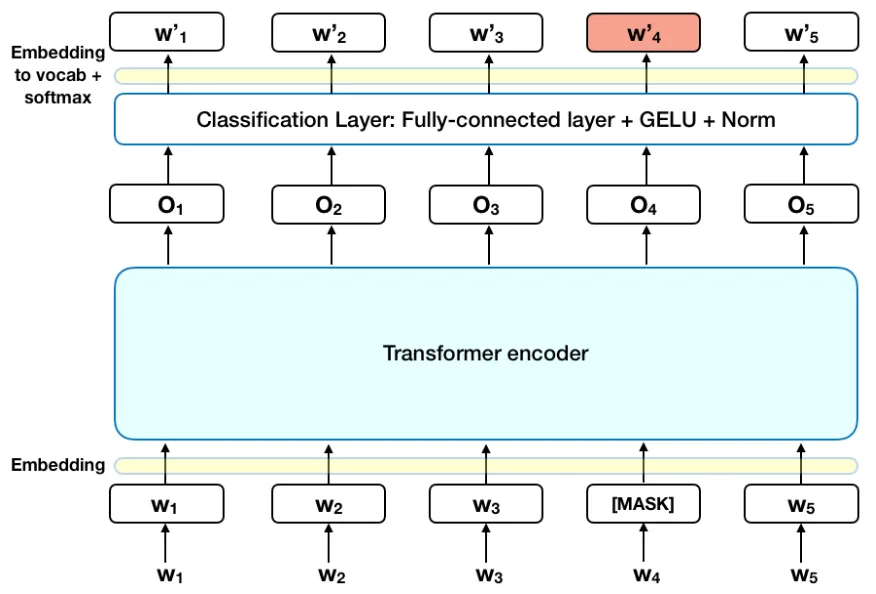
BERT model
Bidirectional Encoder Representations from Transformers (BERT) is an encoder-only model trained in a self-supervised way.
We mask some of the tokens, and then predict them.
Next-Sentence-prediction
Another loss is next sentence prediction: the model receives two sentences and tries to predict if the next sentence is continuation of the first one.
[CLS] token is inserted before the first sentence and [SEP] token is inserted between two sentences.
BERT summary
- We train on Masked reconstruction and next-sentence-prediction loss
- As a result we get good encodings
- These encodings can be used in downstream tasks
- One of the main applications is search: we can map documents to $512$-dimensional vectors. The search is then just nearest neighbours search.
#!pip install transformers
#import transformers
from transformers import pipeline
unmasker = pipeline('fill-mask', model='bert-base-uncased')
unmasker("Artificial Intelligence [MASK] take over the world.")
Some weights of the model checkpoint at bert-base-uncased were not used when initializing BertForMaskedLM: ['cls.seq_relationship.weight', 'cls.seq_relationship.bias']
- This IS expected if you are initializing BertForMaskedLM from the checkpoint of a model trained on another task or with another architecture (e.g. initializing a BertForSequenceClassification model from a BertForPreTraining model).
- This IS NOT expected if you are initializing BertForMaskedLM from the checkpoint of a model that you expect to be exactly identical (initializing a BertForSequenceClassification model from a BertForSequenceClassification model).
[{'score': 0.8617352843284607,
  'token': 2515,
  'token_str': 'does',
  'sequence': 'artificial intelligence does not take over the world.'},
 {'score': 0.06553470343351364,
  'token': 2097,
  'token_str': 'will',
  'sequence': 'artificial intelligence will not take over the world.'},
 {'score': 0.026606494560837746,
  'token': 2106,
  'token_str': 'did',
  'sequence': 'artificial intelligence did not take over the world.'},
 {'score': 0.010828700847923756,
  'token': 2064,
  'token_str': 'can',
  'sequence': 'artificial intelligence can not take over the world.'},
 {'score': 0.009001809172332287,
  'token': 2071,
  'token_str': 'could',
  'sequence': 'artificial intelligence could not take over the world.'}]
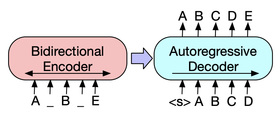
Encoder-decoder models
There are architectures that try to combine encoder and decoder, for example, BART which combines bidirectional and autoregressive transformers:
We can do transformations to the input.
Huggingface
https://huggingface.co/ hosts a huge amount of NLP transformer models and many different pipelines.
Memory and complexity
Attention scales like $L^2$ where $L$ is the sequence length. For very long sequences it will be time consuming, so quite a long of fast attention variants have been proposed.
For language models, the attention is not the main bottleneck.
Most of the parameters are located in feedforward layers that map $N_f \rightarrow 4 N_f$.
They need to be compressed, quantized, etc.
Recent leaks of LLAMA and related models, people try to quantize them but do not systematically check the accuracy.
Summary
- Classical autoregressive models
- Concept of attention
- Transformer architecture
Next lecture: Vision Transformer models
- Original idea of VIT
- Different applications of VIT to classical image tasks
- Modern trends: MobileVIT, CrossVIT