Lecture 7: Graph Neural Networks

Previous lecture: Visition Transformers

• Original idea of VIT
• Beit (3 versions)
• Cait
• Cross-ViT
• SWIN
• Transformers for object detection
• DINO
• MobileVIT (3 versions)
• XCiT
• MLP-Mixer

Graph Neural Networks

• Deep learning on graphs
• Basic models
• Applications

What is a graph

So far, we have discussed images and sequences. There are applications, where the data can be shown as a graph.

A graph represents the relations (edges) between a collection of entities (nodes or vertices).

Basic concepts include adjacency matrix of the graph.

A sequence can be thought a particular case of the linear graph.

Can we think about some particular applications of graphs?

What features can we find in graphs

Graphs in Data Science comes with different attributes:

• Vertex (Node) attributes: what is this node type, or something computed from the graph such as number of neighbours
• Edge (or link) attributes: what is this link type (edge identity), weight of the edge
• Global attributes:: number of nodes, longest path

What kind of problems we need to solve with graphs

• Graph classification (given many samples of graphs, classify them)
• Node classification
• Link prediction

Graph-level task

For these tasks, our goal is to predict a property of a given graph as a whole.

For example, this can be molecule classification: is this molecule toxic? How does it smell?

The main challenge is the same as with text classification: the input data has different sizes, and the architecture should output the vector of the same size.

Graph-level tasks are similar to image classification.

Node-level

We need to predict some property of each node of the graph. For example, we recommend the product or we don't recommend the product in recommender systems.

Node-level tasks are similar to image segmentation tasks.

Edge-level

We can also try to assign some labels/output to each edge of the graph.

This can also be link prediction: given two nodes determine, if there is an edge between them or not.

Applications of GNN

• social networks
• recommendation systems
• drug discovery
• NP-complete optimization problems on graphs (logistics, even quantum computing).
• Computer vision tasks, point clouds.

Graph data (1)

Molecules can be characterized as graphs, and now it is one of the main tools to build drug design networks.

Graph data (2)

• Social networks as graphs
• Citation networks as graphs

How to represent graphs

• Representing the graphs using adjacency matrix is ok for small graphs.
• We can apply CNN on such matrices on images

1. Such approach scales badly with the number of vertices: many graphs have million of vertices!
2. Many adjacency matrices can encode the same graph (permutation of vertices!).

Also, how to treat graphs of different sizes?

Spectral convolutions on graphs

Let $A$ be the adjacency matrix of the graph, and $L$ be the normalized graph Laplacian of this graph,

$$L = I - D^{-1/2} A D^{-1/2} = U \lambda U^{\top}, \quad D = \sum_j A_{ij}.$$

A standard convolution operator can be thought as elementwise multiplication in the frequency domain:

$$g_{\theta} \bigstar x = U g_{\theta}(\Lambda) U^{\top},$$

where $U$ is a Fourier transform and $g(\theta)$ is applied to the eigenvalues of the normalized graph Laplacian.

The transformation $U^{\top} x$ is called graph Fourier transform.

How we can get standard convolution using this notation?

Two different approaches

There are two different ways to build graph neural networks.

1. Convolutional Neural Networks on Graphs with Fast Localized Spectral Filtering, Michaël Defferrard, Xavier Bresson, Pierre Vandergheynst
2. Semi-supervised classification with graph convolutional neural networks, Kipf, Welling

The first one uses spectral convolutions, the second one proposes to use adjacency matrix for mixing the information between different nodes.

ChebNet

The paper with spectral convolutions was the first.

The idea is to apply polynomial filters as

$$g_{\theta} \bigstar x = U g_{\theta}(\Lambda) U^{\top},$$$$g_{\theta}(\Lambda) = \sum_{k=0}^{K-1} \theta_k \Lambda^k.$$

What is the analogue of the receptive field for such kind of convolution?

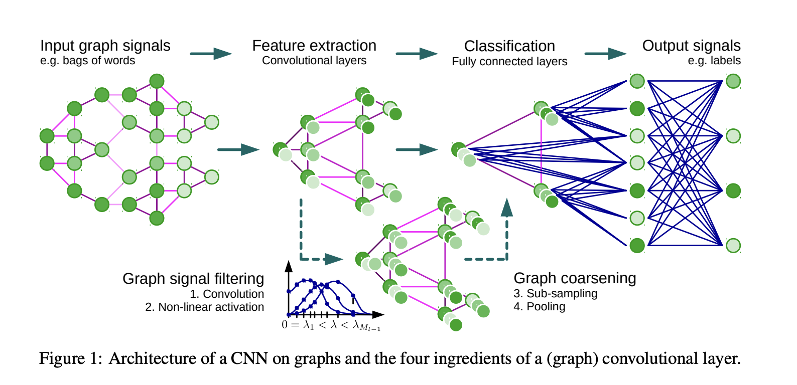
ChebNet

Instead of monomials, one can use Chebyshev polynomials instead, parametrizing the convolution with the Chebyshev coefficients.

$$g_{\theta}(\Lambda) = \sum_{k=0}^{K-1} c_k T_k(\Lambda).$$

Application of such filter to a signal can be done in $\mathcal{O}(K)$ matrix-by-vector products with the matrix $L$.

A signal is a vector defined in each node of the graph!

Then, the paper proposes to use Pooling by simple graph coarsening technique.

\begin{equation} \text{Choose unmarked vertex } i, \text{and match it with an unmarked neighbor } j \\ \text{such that } W_{ij} \left(\frac{1}{d_i} + \frac{1}{d_j}\right) \text{ is maximized} \end{equation}

where $W_{ij}$ is the weight of the edge between vertices $i$ and $j$, $d_i$ and $d_j$ are the degrees of vertices $i$ and $j$, respectively.

Graph convolutional networks

The work of Kimpf and Welling proposes another idea which uses adjacency matrix.

\begin{equation} H^{(l+1)} = \sigma\left(\hat{D}^{-\frac{1}{2}}\hat{A}\hat{D}^{-\frac{1}{2}}H^{(l)}W^{(l)}\right), \quad \hat{A} = I + A, \quad\hat{D}_i = \sum_j \hat{A}_{ij}. \end{equation}

Matrix $\hat{A}$ is the adjacency matrix with added self-connection, $H^{(l)} \in \mathbb{R}^{N \times D}$ is the matrix of activations in the $l$-th layer.

This implements a mapping $f(X, A)$.

We can use this for node classification!

Message passing networks

The models above are node-based, edges are not involved.

We can consider representation where the information is stored as vectors:

• On the nodes
• On the edges

We can then apply MLP to node data; we can also apply MLP to the edge data.

There is no exchange between edges and nodes!

We can do simple global pooling (like averaging).

For more complex interface a message passing mechanism appears.

Message passing networks (2)

In has been proposed in a paper Message passing neural networks in quantum chemistry

The task was predicting the energy of the molecule from its graph.

During the message passing phase, hidden states $h^t_u$ at each node in the graph are updated based on messages $m^{(t+1)}_v$ according to

\begin{align*} m_{t+1}^v &= \sum_{w\in N(v)} M_t(h_t^v, h_t^w, e_{vw}) \\ h_{t+1}^v &= U_t(h_t^v, m_{t+1}^v) \end{align*}

Then, we can collect the features for the graph.

Functions $M$, $U$ are learnable functions.

Attention in graphs

Graph Attention Networks Petar Veličković, Guillem Cucurull, Arantxa Casanova, Adriana Romero, Pietro Liò, Yoshua Bengio

Proposes graph variant of attention mechanism.

It is very natural to look for attention mechanism, because it allows for variable-size input.

The attention is computed only for the neighbours in a graph using the standard self-attention block.

$$\alpha_{ij}=\frac{\exp(e_{ij})}{\sum_{k\in N_i}\exp(e_{ik})}$$

Then we take a linear combintation with those features.

Summary

A typical GNN does

a) Independent node transformations

b) Aggregation of the node features in the form of message passing or coarsening of the graph.

GIN architecture (and how powerful are GNN)

How Powerful are Graph Neural Networks? Keyulu Xu, Weihua Hu, Jure Leskovec, Stefanie Jegelka

This paper starts from a question: can the graph neural networks distiguish two isomorphic graphs?

This will help to show expressiveness of GNN architecture.

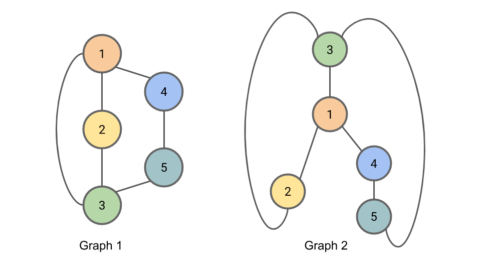
What is graph isomorphism

The graph isomorphism problem asks whether two graphs are topologically identical. No polynomial-time algorithm is known for this task.

Definition: two graphs are considered isomorphic if there is a mapping between the nodes of the graphs that preserves node adjacencies

Weisfeiler-Lehman (WL) test of graph isomorphism has been proposed in 1968 is an effective and computationally efficient test that works for large set of graphs.

Weisfeiler-Lehman test

The WL algorithm produces for each graph its canonical form. If the canonical forms are different, the two graphs are definitely different.

• For iteration of the algorithm we will be assigning to each node a tuple $L_{i, n}$ containing the node’s old compressed label and a multiset of the node’s neighbors' compressed labels. A multiset is a set (a collection of elements where order is not important) where elements may appear multiple times.
• At each iteration we will additionally be assigning to each node a new “compressed” label $C_{i, n}$ for that node’s set of labels. Any two nodes with the same $L_{i, n}$ will get the same compressed label.

Algorithm:

• Start with $C_{0, k} = 1$ for all nodes
• Build $L_{i, n}$ as the multiset of the previous compressed label at this node and all neighbouring labels. All nodes with the same $L$ will get the same $C$ (algorithmically, we can store the hash of the set).
• We stop if the number of iterations reached, or the labels do not change.

Note: at the start each node will get the label equal to the degree of the vertex.

Expressive power of GNN

If GNN maps graphs to different embeddings, the WL test does so as well!

(So, we need to find an architecture that is as powerful as WL).

Lemma

Let $G_1$ and $G_2$ be any two non-isomorphic graphs. If a graph neural network $A: G \rightarrow \mathbb{R}^d$ maps $G_1$ and $G_2$ to different embeddings, then the Weisfeiler-Lehman graph isomorphism test also decides that $G_1$ and $G_2$ are not isomorphic.

Opposite result:

For a certain conditions, if WL tests gives positive results, GNN maps to different embeddings.

Let $A : G \rightarrow \mathbb{R}^d$ be a graph neural network (GNN). With a sufficient number of GNN layers, A maps any graphs $G_1$ and $G_2$ that the Weisfeiler-Lehman test of isomorphism decides as non-isomorphic, to different embeddings if the following conditions hold:

• a) A aggregates and updates node features iteratively with

$h^{(k)}_v = \varphi(h^{(k-1)}_v, f(\{h^{(k-1)}_u\}_{u \in N(v)})),$ where the functions f, which operates on multisets, and $\varphi$ are injective.

• b) A's graph-level readout, which operates on the multiset of node features $\{h^{(k)}_v\}_{v \in G}$, is injective.

Graph Isomorphism network (GIN)

The node update reads (theory say with probability one it will work, looks like ResNet-type architecture)

$h^{(k)}_v = \text{MLP}^{(k)}\left((1-\varepsilon_k) h^{(k-1)}_v + \varepsilon_k \sum_{u \in N(v)} h^{(k-1)}_u\right).$

$h_G = \text{CONCAT}\left(\text{READOUT}\left(h^{(k)}_v \mid v \in G \right)\right)_{v \in G, k=0,1,...,K}$

We do not average the inbetween mode features, we stack them alltogether.

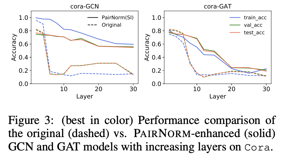
Challenges in Graph Neural Networks

One of the problems in GNN is oversmoothing: the node representations tend to become indistinguishable if the number of layers increase.

In practice, it means that deeper graph networks do not lead to better accuracy.

This problem has been studied by adding residual connections or by the technique known as Dropout (in the context of graph neural networks, DropEdge ).

Also, we can use normalisation (PairNorm).

Still, as far a I know, depth does not help and typically 2-4 layers are used in GNN.

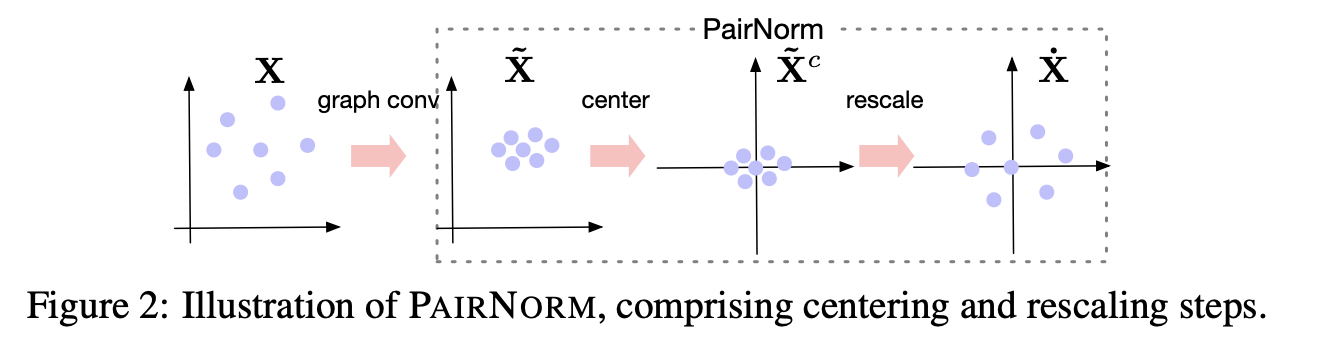
PairNorm

The idea of PairNorm is quite interesting.

The graph convolution can be proposed from the following optimization problem:

$$\min_{\hat{X}} \sum_i \Vert \hat{x}_i - x_i \Vert^2 + \sum_{(i, j) \in E} \Vert \hat{x}_i - \hat{x}_j \Vert^2,$$

the solution gives the graph Laplacian.

The problem is that after such transformation, the node embeddings become closer within a cluster.

The PairNorm normalized $\hat{X}$ in such a way that the total sum of squares of distances remains unchanged!

Combinatorial optimization with GNN

One of the most interesting applications of GNN is combinatorial optimization (see, for example review)

For example: traveling salesman problem. How we can use machine learning for it?

Idea

Use supervised learning!

The first idea was a Pointer Network (PtrNet) by Vinyals et. al who mapped a two-dimensional point cloud to an optimal tour.

We collect graphs and optimal tours, and learn the mapping in a supervised way!

Another idea: compute the probability of the edge to be in the tour. Then use beam search to find the optimal one.

Software for GNN

PyG: https://www.pyg.org/

Deep Graph Library: https://www.dgl.ai/

PyG is mostly a collection of fast re-implementations of existing models (with custom sparse ops). DGL introduces a useful higher-level abstraction, allowing for auto-batching (but is somewhat slower).

We covered the basic stuff only...

Much more operations with the links to the papers can be found here:

https://pytorch-geometric.readthedocs.io/en/latest/cheatsheet/gnn_cheatsheet.html

Summary

• Deep learning on graphs
• Basic models
• Applications

Next lecture: General tricks for efficient training:

• Initialization (talked already a little bit)
• Data augmentation
• Neural network compression/pruning
• Clipping
• multi-precision training
• simple distributed training primitives